409 WSN Coverage: Problem Types
409.1 Learning Objectives
By the end of this chapter, you will be able to:
- Formulate Area Coverage Problems: Define and solve continuous 2D region monitoring challenges
- Design Point Coverage Solutions: Optimize sensor placement for discrete critical location monitoring
- Implement Barrier Coverage: Create effective intrusion detection systems using k-barrier coverage
- Calculate Coverage Metrics: Compute coverage ratio, k-coverage requirements, and sensor density
- Apply Coverage Formulations: Select the appropriate coverage type for real-world applications
What is this chapter? This chapter explains the three main types of coverage problems in WSN: area coverage, point coverage, and barrier coverage.
Key Concepts:
| Coverage Type | What it Monitors | Example Application |
|---|---|---|
| Area Coverage | Continuous 2D region | Environmental monitoring |
| Point Coverage | Discrete critical points | Building access control |
| Barrier Coverage | Border/perimeter crossing | Border surveillance |
Why This Matters: - Different applications need different coverage approaches - Cost optimization depends on coverage type selection - Redundancy requirements vary by application criticality
409.2 Prerequisites
Before diving into this chapter, you should be familiar with:
- WSN Coverage: Core Concepts: Understanding of coverage fundamentals, sensing models, and the Zhang-Hou theorem
- WSN Overview: Fundamentals: Basic WSN architecture and design constraints
409.3 Coverage Problem Types
409.3.1 Area Coverage
Objective: Monitor every point in a continuous 2D region.

{fig-alt=“Area coverage model flowchart showing target area A monitored by four sensors (Sensors 1-4), their coverage areas combining into a union (∪Cᵢ), a decision node checking if area A is subset of union, leading to either complete coverage (green, minimize active sensors) or coverage holes (red, deploy more sensors)”}
Applications: - Environmental monitoring (temperature, humidity) - Precision agriculture (soil conditions) - Indoor climate control - Pollution tracking
Challenge: Minimize number of active sensors while ensuring complete coverage.
Mathematical Formulation:
Let \(A\) be the region to monitor, and \(C_i\) be the coverage disk of sensor \(i\) with radius \(R_s\):
\[ A \subseteq \bigcup_{i \in \text{Active}} C_i \]
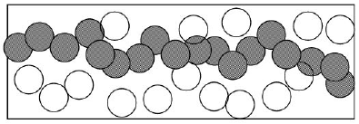
Energy-Efficient Approach:
Deploy redundant sensors (many more than needed), then use duty cycling:
Rotation Schedule:
To maximize lifetime, rotate active sensors:
Round 1: Sensors {1, 3, 5, 7} active (cover 100%)
Round 2: Sensors {2, 4, 6, 8} active (cover 100%)
Round 3: Back to {1, 3, 5, 7}
...
Lifetime Improvement: If 50% of sensors needed for coverage, lifetime doubles through rotation.
409.3.2 Point Coverage
Objective: Monitor a discrete set of critical points (not continuous area).

{fig-alt=“Point coverage model showing four orange points of interest (door, window, valve, junction) monitored by three teal sensors with overlapping coverage (dotted lines). Sensor 1 covers Points 1-2, Sensor 2 covers Points 2-3, Sensor 3 covers Points 3-4, resulting in successful complete point coverage (green) rather than adding more sensors (red).”}
Applications: - Building access monitoring (doors, windows) - Pipeline monitoring (junctions, valves) - Bridge structural health monitoring (stress points) - Smart grid (critical substations)
Mathematical Formulation:
Let \(P = \{p_1, p_2, ..., p_n\}\) be points to cover:
\[ \forall p_i \in P, \exists s_j \in \text{Active} : d(p_i, s_j) \leq R_s \]
Minimum Sensor Placement:
This is the classic set cover problem (NP-hard):
Redundancy for Reliability:
Critical applications require k-coverage: every point covered by at least k sensors (fault tolerance).
1-coverage: Each point monitored by ≥1 sensor
2-coverage: Each point monitored by ≥2 sensors (tolerates 1 failure)
k-coverage: Each point monitored by ≥k sensors (tolerates k-1 failures)The Misconception: If coverage analysis shows 100%, the entire area is monitored.
Why It’s Wrong: - 1-coverage means ONE sensor sees each point (single point of failure) - Sensor failure creates instant blind spot - Sensing range is idealized (obstacles, interference reduce actual range) - Temporal coverage differs from spatial (duty cycling creates gaps)
Real-World Example: - Security system: 100% 1-coverage of warehouse - One sensor battery dies: 15% of area now unmonitored - Intruder enters through dead zone: Undetected - With 2-coverage: Still 100% covered after one failure
The Correct Understanding: | Coverage Type | Meaning | Use Case | |————–|———|———-| | 1-coverage | Every point seen by ≥1 sensor | Non-critical monitoring | | 2-coverage | Every point seen by ≥2 sensors | Fault tolerance | | k-coverage | Every point seen by ≥k sensors | Critical applications | | Probabilistic | Statistical coverage guarantee | Resource-constrained |
Specify k-coverage requirements explicitly. “100% coverage” is meaningless without k value.
409.3.3 Barrier Coverage
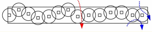
Objective: Detect intruders crossing a barrier (line or belt).

{fig-alt=“Barrier coverage linear deployment showing four teal sensors positioned sequentially along border from start to end, with overlapping coverage zones (light green). Red intruder path crosses through Sensor 2 and Sensor 3 coverage zones, demonstrating guaranteed detection along the barrier perimeter.”}
Applications: - Border surveillance - Perimeter security (military bases, critical infrastructure) - Wildlife corridor monitoring - Pipeline intrusion detection
k-Barrier Coverage Levels:

{fig-alt=“K-barrier coverage taxonomy showing barrier coverage root splitting into three levels: 1-barrier (teal, basic detection, perimeter monitoring), 2-barrier (orange, redundant detection, critical infrastructure with weak path-crossing and strong every-point variants showing sensor trade-offs), and k-barrier (red, high security, military borders)”}
Weak vs. Strong Barrier:
Weak k-Barrier:
: Every path crossing the barrier intersects sensing ranges of at least k sensors
Strong k-Barrier:
: Every point on every path crossing the barrier is within sensing range of at least k sensors simultaneously
Deployment Strategy:
For a barrier of length \(L\) with sensors of range \(R_s\):
Minimum sensors for 1-barrier: \(\lceil L / (2R_s) \rceil\)
Minimum sensors for k-barrier: Approximately \(k \times \lceil L / (2R_s) \rceil\)
409.4 Coverage Type Comparison
| Aspect | Area Coverage | Point Coverage | Barrier Coverage |
|---|---|---|---|
| Objective | Monitor continuous region | Monitor discrete points | Detect crossing intruders |
| Complexity | Medium | NP-hard (set cover) | Linear in barrier length |
| Sensor Count | High (area-dependent) | Moderate (point-dependent) | Low (linear deployment) |
| Redundancy | Overlap regions | Multiple sensors per point | Multiple barrier layers |
| Application | Environmental, agriculture | Access control, structural | Border, perimeter security |
| Energy Efficiency | Duty cycling effective | Sleep scheduling per point | Barrier rotation possible |
409.5 Summary
This chapter covered the three main coverage problem types in Wireless Sensor Networks:
- Area Coverage: Monitors continuous 2D regions, requires coverage union to contain entire target area, benefits from duty cycling with redundant deployment
- Point Coverage: Monitors discrete critical points, formulated as NP-hard set cover problem, supports k-coverage for fault tolerance
- Barrier Coverage: Detects intruders crossing boundaries, with weak k-barrier (paths cross k sensors) and strong k-barrier (every point covered by k sensors)
- K-Coverage Selection: Life-critical applications need k≥3, infrastructure uses k=2, environmental monitoring accepts k=1
- Cost-Coverage Trade-off: Higher k-coverage requires more sensors but provides fault tolerance and reliability
409.6 Knowledge Check
409.7 What’s Next
The next chapter presents WSN Coverage Worked Examples, with detailed k-coverage analysis for critical infrastructure, duty cycling energy budgets, sensing range trade-off calculations, and an interactive coverage playground for hands-on experimentation.