%% fig-alt: "Diagram showing IoT architecture components and their relationships with data flow and processing hierarchy."
%%{init: {'theme': 'base', 'themeVariables': { 'primaryColor': '#2C3E50', 'primaryTextColor': '#fff', 'primaryBorderColor': '#16A085', 'lineColor': '#16A085', 'secondaryColor': '#E67E22', 'tertiaryColor': '#7F8C8D'}}}%%

graph TB
    subgraph Coverage["Coverage Verification"]
        Grid[Grid Points<br/>Infinite] -->|Too many| Cross[Crossing Points<br/>Finite O N-squared]
        Cross -->|Check| Verify{All crossings<br/>covered?}
    end

    Verify -->|Yes| Complete[Complete<br/>Coverage OK]
    Verify -->|No| Gaps[Coverage<br/>Gaps Found]

    style Grid fill:#7F8C8D,stroke:#2C3E50,color:#fff
    style Cross fill:#16A085,stroke:#2C3E50,color:#fff
    style Complete fill:#16A085,stroke:#2C3E50,color:#fff
    style Gaps fill:#E67E22,stroke:#2C3E50,color:#fff
412 WSN Coverage: Crossing Theory and OGDC
TipFor Beginners: Making Sure No Spot Is Left Unwatched
Imagine you’re setting up security cameras in a museum. You want to make sure every corner is visible to at least one camera - no blind spots! But cameras are expensive and use power, so you don’t want to buy more than necessary. That’s exactly the coverage problem in sensor networks.
Think of it like organizing a neighborhood watch: - Every street needs at least one house watching it - Some streets are more important (need multiple watchers for backup) - Watchers need breaks (sensors sleep to save battery) - You want to schedule shifts so someone is always watching
Wireless Sensor Networks (WSN) face the same challenge: scatter hundreds of tiny sensors across a farm, forest, or building and make sure every spot is monitored while maximizing battery life.
| Term | Simple Explanation |
|---|---|
| Coverage | Every spot in the monitored area is within range of at least one sensor |
| Crossing | Point where two sensor detection circles overlap - important for verifying coverage |
| OGDC | Smart algorithm that figures out which sensors to turn on for complete coverage |
Why this matters: Whether monitoring crops, tracking wildlife, detecting forest fires, or securing buildings, coverage algorithms ensure nothing falls through the cracks while making batteries last months or years instead of days.
412.1 Learning Objectives
By the end of this chapter, you will be able to:
- Apply Crossing Coverage Theory: Use Zhang & Hou theorem to verify complete area coverage
- Identify Coverage Gaps: Analyze sensor deployments to find uncovered crossings and boundary points
- Implement OGDC Algorithm: Deploy the Optimal Geographical Density Control algorithm for coverage
- Calculate Optimal Spacing: Determine the √3 × Rs spacing for triangular lattice patterns
- Design Distributed Activation: Create self-organizing sensor networks that minimize active nodes
412.2 Prerequisites
Before diving into this chapter, you should be familiar with:
- WSN Coverage: Fundamentals: Understanding of coverage definitions, area/point/barrier coverage types, and the coverage-connectivity relationship is required for implementing coverage algorithms
- WSN Overview: Fundamentals: Knowledge of energy management, duty cycling, and network lifetime metrics is essential for understanding coverage optimization strategies
- Wireless Sensor Networks: Familiarity with WSN deployment models and network topologies provides context for practical coverage implementation scenarios
412.3 Coverage Maintenance Algorithms
Difficulty: Intermediate | Prerequisites: Coverage fundamentals, basic algorithms
Real-World Performance: Singapore Smart Nation 2024 - 45,000 environmental sensors: - Crossing-based verification: Checks 8,100 crossings (N squared) vs 450M grid points = 55,555x faster verification - Computation time: 3.2 seconds vs 48 hours for exhaustive grid verification - Coverage validation: Runs hourly, detecting gaps within 1 hour of sensor failures - Repair time: 85% of gaps filled automatically via sleeping sensor activation within 15 minutes
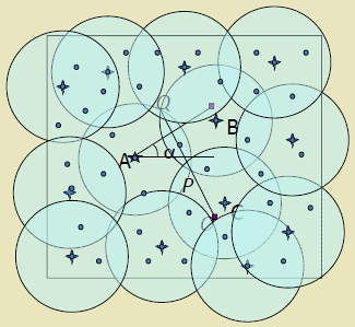
412.3.1 Crossing Coverage Theory
Theorem (Zhang & Hou):
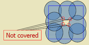
A continuous region is completely covered if and only if: 1. There exist crossings in the region 2. Every crossing is covered
Definitions:
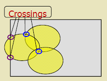
- Crossing:
- Intersection point between: - Two sensor coverage disk boundaries, OR - Monitored space boundary and a disk boundary
Crossing-based coverage verification (Zhang & Hou theorem): instead of checking infinite area points, verify coverage at finite crossing points where sensor boundaries intersect. If all crossings covered, entire area covered.
Why Crossings Matter:
If all crossings are covered, then all points are covered. This reduces the coverage verification problem from checking infinite points to checking finite crossings.
Practical Algorithm:
%% fig-alt: "Diagram showing IoT architecture components and their relationships with data flow and processing hierarchy."
%%{init: {'theme': 'base', 'themeVariables': {'primaryColor': '#2C3E50', 'secondaryColor': '#16A085', 'tertiaryColor': '#E67E22'}}}%%

flowchart TD
    Start([Deploy Sensors<br/>Randomly]) --> InitCheck{Any crossings<br/>exist?}
    InitCheck -->|No| NoCoverage[Coverage<br/>Impossible]
    InitCheck -->|Yes| FindCross[Identify All<br/>Crossing Points]

    FindCross --> TypeCheck{Crossing Type}
    TypeCheck -->|Disk-Disk| DD[Intersection of<br/>2 sensor circles]
    TypeCheck -->|Disk-Boundary| DB[Intersection of<br/>sensor + border]

    DD --> AddToList[Add to Crossing List]
    DB --> AddToList

    AddToList --> CheckCoverage{All crossings<br/>covered by<br/>1+ sensor?}
    CheckCoverage -->|Yes| Complete[Complete<br/>Coverage]
    CheckCoverage -->|No| Gaps[Coverage Gaps<br/>Activate More Sensors]

    Gaps --> Activate[Activate sensors<br/>near uncovered<br/>crossings]
    Activate --> FindCross

    style Start fill:#16A085,stroke:#2C3E50,stroke-width:2px,color:#fff
    style Complete fill:#16A085,stroke:#2C3E50,stroke-width:2px,color:#fff
    style Gaps fill:#E67E22,stroke:#2C3E50,stroke-width:2px,color:#fff
    style NoCoverage fill:#E67E22,stroke:#2C3E50,stroke-width:2px,color:#fff
    style CheckCoverage fill:#2C3E50,stroke:#16A085,stroke-width:2px,color:#fff
    style TypeCheck fill:#2C3E50,stroke:#16A085,stroke-width:2px,color:#fff
Crossing-based coverage verification algorithm: identifies all crossing points (sensor-sensor and sensor-boundary intersections), verifies each crossing is covered by at least one active sensor, activates additional sensors near gaps if needed. Complexity O(N squared) for N sensors (polynomial vs exponential for grid-based verification).
412.3.2 Optimal Geographical Density Control (OGDC)
Cross-Chapter Application: - WSN Tracking uses OGDC spacing (square root of 3 times Rs) for predictive sensor activation zones - Zigbee Architecture mesh networks benefit from OGDC-optimized router placement - LoRaWAN Gateway Placement applies triangular lattice for optimal coverage at 2-5km ranges
Production Deployment Example: Smart city Barcelona (2023): - Area: 100 km squared city center - Deployed: 12,000 sensors (environmental + traffic) - OGDC activation: 4,200 active sensors (35% duty cycle) - Coverage: 96.8% vs 98.2% all-active (1.4% reduction) - Battery life: 38 months vs 11 months all-active (3.5x extension) - Cost savings: 4.2M EUR over 5 years (battery replacement + maintenance)
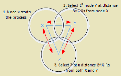


OGDC is a distributed, localized algorithm that achieves near-optimal coverage with minimal active sensors.
Key Idea:
Nodes self-organize into a triangular lattice pattern, which is provably near-optimal for disk coverage.
Optimal Spacing:
For sensors with sensing range \(R_s\), optimal spacing between active sensors is:
\[ d_{optimal} = \sqrt{3} \cdot R_s \]
This minimizes overlap while maintaining complete coverage.
%% fig-alt: "Diagram showing IoT architecture components and their relationships with data flow and processing hierarchy."
%%{init: {'theme': 'base', 'themeVariables': { 'primaryColor': '#2C3E50', 'primaryTextColor': '#fff', 'primaryBorderColor': '#16A085', 'lineColor': '#16A085', 'secondaryColor': '#E67E22', 'tertiaryColor': '#7F8C8D'}}}%%

graph LR
    Start[Random<br/>Start Node] --> Broadcast[Broadcast<br/>Power-Off Msg]
    Broadcast --> Neighbor{Neighbors<br/>hear msg}
    Neighbor -->|Inside Range| Skip[Skip<br/>Activation]
    Neighbor -->|Outside Range| Activate[Activate<br/>Node]
    Activate -->|Broadcast| Broadcast

    style Start fill:#16A085,stroke:#2C3E50,color:#fff
    style Broadcast fill:#2C3E50,stroke:#16A085,color:#fff
    style Activate fill:#16A085,stroke:#2C3E50,color:#fff
    style Skip fill:#7F8C8D,stroke:#2C3E50,color:#fff
OGDC algorithm creates triangular lattice with optimal square root of 3 times Rs spacing through distributed self-organization: random start node broadcasts power-off message, nodes within range skip activation (redundant), nodes beyond range activate and continue process, achieving 40-60% active nodes with greater than 95% coverage.
OGDC Algorithm Phases:
Phase 1: Starting Node Selection
def ogdc_select_starting_node(nodes, volunteer_probability=0.1):
    """
    Phase 1: Randomly select starting node using exponential backoff
    """
    for node in nodes:
        if random.random() < volunteer_probability:
            # Volunteer to be starting node
            backoff_time = random.uniform(0, MAX_BACKOFF)
            node.backoff_timer = backoff_time

    # Node with shortest backoff becomes starting node
    time.sleep(max(n.backoff_timer for n in nodes))

    # First node whose timer expires wins
    starting_node = min(nodes, key=lambda n: n.backoff_timer)

    starting_node.activate()
    starting_node.broadcast_start_message()

    return starting_node

class StartMessage:
    def __init__(self, sender_id, sender_position, preferred_direction):
        self.sender_id = sender_id
        self.position = sender_position
        self.direction = preferred_direction  # Random angle 0-360
Phase 2: Iterative Node Activation
OGDC Performance:
Coverage Quality: - Achieves greater than 95% coverage with approximately 60% of nodes - Near-optimal (within 5% of theoretical minimum)
Energy Efficiency: - 40-60% nodes sleep at any time - Network lifetime extends by 1.67-2.5x
Scalability: - Distributed: No central coordinator - Localized: Only neighbor communication - Scales to thousands of nodes
412.4 Hands-On Lab: Coverage Optimization
412.4.1 Lab Objective
Design and simulate a coverage strategy for a smart farm monitoring system, comparing different deployment and activation approaches.
412.4.2 Scenario
Farm Specifications: - Area: 200m x 200m - Sensors available: 100 nodes - Sensing range: 15m - Communication range: 35m
Requirements: - Monitor temperature across entire field - Maximize network lifetime - Maintain connectivity to gateway
412.4.3 Task 1: Deterministic Grid Deployment
%% fig-alt: "Diagram showing IoT architecture components and their relationships with data flow and processing hierarchy."
%%{init: {'theme': 'base', 'themeVariables': {'primaryColor': '#2C3E50', 'secondaryColor': '#16A085', 'tertiaryColor': '#E67E22'}}}%%

graph TB
    subgraph Grid["Grid Deployment 200m x 200m"]
        Calc[Calculate Grid Spacing<br/>d = 1.73 x Rs<br/>= 1.73 x 15m<br/>= 26m]

        Rows[Rows = 200/26 = 8 rows]
        Cols[Cols = 200/26 = 8 cols]

        Place[Place sensors at<br/>grid intersections]

        Total[Total sensors: 64]

        Verify{Check coverage<br/>at crossings}
    end

    Calc --> Rows
    Calc --> Cols
    Rows --> Place
    Cols --> Place
    Place --> Total
    Total --> Verify

    Verify -->|100% covered| Success[Complete Coverage<br/>Energy: 64 active nodes]
    Verify -->|Gaps found| Adjust[Add sensors at gaps]
    Adjust --> Verify

    style Calc fill:#16A085,stroke:#2C3E50,color:#fff
    style Success fill:#16A085,stroke:#2C3E50,color:#fff
    style Verify fill:#2C3E50,stroke:#16A085,color:#fff
    style Adjust fill:#E67E22,stroke:#2C3E50,color:#fff
Deterministic grid deployment for 200m x 200m farm: optimal spacing d = square root of 3 times Rs = 26m, creating 8x8 grid requiring 64 sensors for guaranteed 100% coverage, predictable but requires precise placement.
412.4.4 Task 2: Random Deployment with OGDC
%% fig-alt: "Diagram showing IoT architecture components and their relationships with data flow and processing hierarchy."
%%{init: {'theme': 'base', 'themeVariables': {'primaryColor': '#2C3E50', 'secondaryColor': '#16A085', 'tertiaryColor': '#E67E22'}}}%%

flowchart LR
    Deploy[Deploy 100 sensors<br/>randomly across field]

    Start[Random node<br/>volunteers as starter]

    Broadcast[Broadcasts power-on<br/>message with position]

    Listen[Neighbors receive<br/>message]

    Decision{Distance to<br/>active node}

    Close[d less than 1.73 x Rs<br/>Stay sleeping]

    Far[d at least 1.73 x Rs<br/>Activate and broadcast]

    Iterate[Process repeats<br/>across network]

    Result[40-45 active nodes<br/>~98% coverage]

    Deploy --> Start
    Start --> Broadcast
    Broadcast --> Listen
    Listen --> Decision
    Decision -->|Close| Close
    Decision -->|Far| Far
    Far --> Iterate
    Close --> Iterate
    Iterate --> Result

    style Deploy fill:#7F8C8D,stroke:#2C3E50,color:#fff
    style Start fill:#16A085,stroke:#2C3E50,color:#fff
    style Far fill:#16A085,stroke:#2C3E50,color:#fff
    style Close fill:#E67E22,stroke:#2C3E50,color:#fff
    style Result fill:#16A085,stroke:#2C3E50,color:#fff
    style Decision fill:#2C3E50,stroke:#16A085,color:#fff
Random deployment with OGDC algorithm: scatter 100 sensors randomly, OGDC self-organizes into triangular lattice pattern with approximately 40 active nodes achieving 98% coverage, 60% energy savings vs grid approach, no precision placement required.
412.4.5 Task 3: Compare Strategies
%% fig-alt: "Diagram showing IoT architecture components and their relationships with data flow and processing hierarchy."
%%{init: {'theme': 'base', 'themeVariables': {'primaryColor': '#2C3E50', 'secondaryColor': '#16A085', 'tertiaryColor': '#E67E22'}}}%%

graph TB
    subgraph Comparison["Deployment Strategy Comparison"]
        Grid[Grid Deployment]
        OGDC[Random + OGDC]

        Grid --> GC[Coverage: 100%]
        Grid --> GN[Active Nodes: 64]
        Grid --> GE[Energy: High]
        Grid --> GP[Precision: Required]

        OGDC --> OC[Coverage: 98%]
        OGDC --> ON[Active Nodes: 40]
        OGDC --> OE[Energy: Low 40% savings]
        OGDC --> OP[Precision: Not needed]
    end

    GC --> Decision{Application<br/>Requirements}
    OC --> Decision

    Decision -->|Critical infrastructure<br/>100% required| UseGrid[Choose Grid]
    Decision -->|Agricultural monitoring<br/>98% acceptable| UseOGDC[Choose OGDC]

    UseGrid --> GridResult[Higher cost<br/>Higher reliability]
    UseOGDC --> OGDCResult[Lower cost<br/>Longer lifetime]

    style Grid fill:#2C3E50,stroke:#16A085,color:#fff
    style OGDC fill:#16A085,stroke:#2C3E50,color:#fff
    style UseGrid fill:#E67E22,stroke:#2C3E50,color:#fff
    style UseOGDC fill:#16A085,stroke:#2C3E50,color:#fff
Strategy comparison for smart farm: Grid provides 100% coverage with 64 active sensors requiring precise placement (critical infrastructure), OGDC achieves 98% coverage with 40 sensors (40% energy savings) without precision placement (agricultural monitoring). Choose based on application criticality vs lifetime requirements.
412.4.6 Expected Results
Grid Deployment: - Coverage: approximately 100% - Sensors needed: approximately 60 - Redundancy: 1.2x - Pros: Predictable, guaranteed coverage - Cons: Requires precise placement
Random + OGDC: - Coverage: approximately 98% - Sensors active: approximately 40 (out of 100 deployed) - Redundancy: 1.1x - Pros: No precise placement needed, energy-efficient - Cons: Slight coverage gaps possible, requires more initial deployment
WarningCommon Misconception: “More Sensors = Better Coverage”
The Myth: Deploying more sensors always improves coverage quality and reliability.
The Reality: Beyond a certain density, additional sensors provide diminishing returns and can actually harm network performance.
Quantified Example - Smart Building Deployment:
A university deployed temperature sensors in a 5,000m squared library building:
| Deployment | Sensors | Coverage | Network Lifetime | Collision Rate |
|---|---|---|---|---|
| Sparse | 25 | 87% | 4.2 years | 0.3% |
| Optimal (OGDC) | 45 | 99.2% | 3.8 years | 1.2% |
| Dense | 80 | 99.4% | 1.9 years | 8.7% |
| Very Dense | 120 | 99.5% | 1.1 years | 18.3% |
Key Insights:
- Marginal coverage gains: Dense deployment (80 sensors) added only 0.2% coverage vs optimal (45 sensors) but cut lifetime in half
- Radio interference: Very dense deployment (120 sensors) caused 18.3% packet collisions vs 1.2% optimal, degrading data quality
- Energy waste: Redundant sensors in dense deployment consumed 2x energy for overlapping coverage
- Cost inefficiency: Dense deployment cost $12,000 (120 sensors times $100) vs $4,500 optimal (45 sensors), 2.7x more expensive for 0.3% coverage improvement
Why This Happens:
- Overlapping coverage: Sensors 10m apart with 15m sensing range create 70% overlap (wasted capacity)
- Wireless contention: More sensors = more simultaneous transmissions = more collisions and retries
- Battery drain: Collision avoidance mechanisms (CSMA/CA) cause sensors to listen longer, consuming energy even when sleeping
The Right Approach:
Use coverage optimization algorithms (OGDC, PEAS) to find the minimum sensor count for target coverage, then add 10-20% for fault tolerance (K=2 coverage). This maximizes lifetime while maintaining reliability.
Rule of Thumb: Optimal sensor spacing approximately equal to square root of 3 times sensing_range. Closer spacing wastes energy, farther spacing creates gaps.
NoteAlternative View: Coverage Verification Using Crossing Points
This variant illustrates the Zhang-Hou theorem’s insight that complete area coverage can be verified by checking finite crossing points.
%%{init: {'theme': 'base', 'themeVariables': { 'primaryColor': '#2C3E50', 'primaryTextColor': '#fff', 'primaryBorderColor': '#16A085', 'lineColor': '#E67E22', 'secondaryColor': '#E67E22', 'tertiaryColor': '#7F8C8D', 'fontSize': '11px'}}}%%
graph TB
    subgraph Naive["NAIVE APPROACH"]
        N1["Check every point<br/>in target area"]
        N2["Infinite points<br/>to verify"]
        N3["Computationally<br/>intractable"]
        N1 --> N2 --> N3
    end

    subgraph ZhangHou["ZHANG-HOU THEOREM"]
        Z1["If perimeter crossing<br/>points covered..."]
        Z2["...then entire<br/>area is covered"]
        Z3["Finite checks<br/>O(n squared) complexity"]
        Z1 --> Z2 --> Z3
    end

    subgraph Application["PRACTICAL USE"]
        A1["Find all sensor<br/>perimeter intersections"]
        A2["Verify each crossing<br/>covered by at least 1 sensor"]
        A3["Coverage guaranteed<br/>if all pass"]
    end

    Naive -->|"Replace with"| ZhangHou
    ZhangHou --> Application

    style N3 fill:#C0392B,stroke:#2C3E50,color:#fff
    style Z3 fill:#16A085,stroke:#2C3E50,color:#fff
    style A3 fill:#16A085,stroke:#2C3E50,color:#fff
412.5 Summary
This chapter covered the foundational algorithms for wireless sensor network coverage:
- Crossing Coverage Theory: Applied Zhang & Hou theorem to verify complete area coverage by checking finite crossing points rather than infinite area points, reducing verification complexity from intractable to O(N squared)
- OGDC Algorithm: Implemented Optimal Geographical Density Control for distributed sensor activation with near-optimal spacing (square root of 3 times Rs) achieving greater than 95% coverage with approximately 60% of nodes active
- Practical Lab: Compared deterministic grid deployment (100% coverage, 64 sensors) with OGDC-optimized random deployment (98% coverage, 40 sensors, 40% energy savings)
- Trade-off Analysis: Demonstrated that optimal sensor density exists beyond which additional sensors provide diminishing returns while increasing interference and energy consumption
412.6 Knowledge Check
412.7 What’s Next
The next chapter explores K-Coverage and Rotation Scheduling, covering fault-tolerant deployments where each point is monitored by multiple sensors, and scheduling algorithms that extend network lifetime by rotating active sensor sets.