29 Lab: Wireless Propagation
Measure the Site Before Trusting the Link Budget
29.1 In 60 Seconds
This lab turns wireless propagation theory into measurement evidence. You will predict a link with a link budget, collect RSSI, SNR, retries, packet delivery, placement, obstacle, and time evidence at realistic locations, then explain the gap between prediction and field behavior. The goal is not to prove that one reading looks good; it is to decide whether the link still works under the conditions that the deployment will actually see.
29.2 Start With the Story
Start with a sensor that works on the bench but fails after a wall, a shelf, interference, or a longer distance changes the radio path. The core idea in Lab: Wireless Propagation is simple: wireless propagation is about link margin, obstacles, frequency, fading, interference, antennas, and measured delivery rather than hope. This page focuses that idea on Wireless-propagation lab for collecting RSSI, SNR, retries, packet delivery, obstacle, placement, and time-of-day evidence before approving an IoT radio link. In everyday IoT, RSSI, SNR, retries, packet delivery, placement, and fade margin explain why a gateway location or band choice succeeds or fails. Start simple: write the distance, band, obstacles, antenna assumptions, and measured margin before choosing the radio plan.
29.3 Learning Objectives
By the end of this lab, you should be able to:
- Plan a wireless site survey from a link-budget hypothesis.
- Collect repeatable RSSI, SNR, retry, packet-delivery, location, and obstacle evidence.
- Compare measured path behavior with the predicted path-loss model.
- Separate weak coverage, fading, interference, and non-RF delivery symptoms.
- Decide whether to adjust placement, antenna orientation, channel plan, gateway location, or link technology.
- Produce a release record that explains the remaining margin and revalidation trigger.
29.4 Quick Check: Propagation Lab Method
29.5 How It Works: Run A Wireless Propagation Lab
The lab turns a link-budget hypothesis into field evidence.
- Write the hypothesis. Start with expected path, band, gateway, antenna, receiver mode, and predicted margin.
- Measure representative points. Include edge locations, blocked paths, normal mounting height, orientation, and time-of-day conditions.
- Collect delivery and RF evidence. Pair RSSI or received power with SNR, retries, packet delivery, and channel observations when available.
- Retest the mitigation. After changing placement, channel, antenna, or gateway location, repeat the same measurements.
29.6 Incremental Examples
Beginner Example: A single outdoor sensor is measured at the planned mounting point and compared with the link-budget estimate.
Intermediate Example: A building survey maps several rooms, noting walls, device height, RSSI, SNR, and delivery rate.
Advanced Example: An industrial site repeats measurements during quiet and busy periods to separate coverage, fading, and interference risks.
29.7 Concept Check: Representative Point
Why should the lab include the weakest expected location?
Answer: a link that passes near the gateway may still fail at the edge, behind obstacles, or in the actual enclosure and orientation.
29.8 Concept Check: Mitigation Evidence
What must happen after moving an antenna or changing a channel?
Answer: rerun the same measurement record. The mitigation is not proven until the new evidence covers the same scenario.
29.9 Try It Yourself
Draft a site-survey sheet with columns for location, obstacle path, orientation, RSSI, SNR, delivery rate, retry count, mitigation, and retest result.
29.10 See Also
- Radio Wave Basics for IoT - frames the radio terms behind the review loop.
- Path Loss and Link Budgets - provides the hypothesis the lab tests.
- Fading and RF Interference - helps classify failed measurements.
29.11 Lab Setup
You can use any radio platform that exposes at least one signal-strength metric and one delivery metric. A phone Wi-Fi analyzer, gateway diagnostics page, development board, protocol sniffer, packet counter, or site-survey tool can all work. The important part is that you record the same fields at each point.
29.11.1 Required Evidence
RSSI or received power, SNR or link-quality indicator when available, retry count, packet delivery, location, height, orientation, obstacle path, and timestamp.
29.11.2 Optional Evidence
Channel occupancy, noise floor, spectrum snapshot, antenna photo, floor-plan mark-up, gateway load, firmware mode, and weather or occupancy notes.
29.11.3 Boundary
Do not compare RSSI values across radio families without checking receiver sensitivity, data rate, bandwidth, coding, and SNR. RSSI is context, not a universal grade.
29.12 Measurement Discipline
Take several samples at each point. Record minimum, median, and worst observed delivery behavior instead of keeping only the best reading. If the link matters during a busy shift, measure during that shift. If the sensor will be mounted near metal, behind a door, low to the ground, or inside an enclosure, measure that mounted condition.
29.13 Lab Workflow
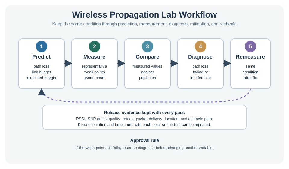
The workflow has five passes:
- Predict the link from the path-loss and link-budget chapter.
- Measure representative points, weak points, and worst-case points.
- Compare the measured values with the prediction.
- Diagnose whether the gap is path loss, fading, interference, placement, or non-RF behavior.
- Remeasure after the mitigation under the same condition that caused concern.
29.14 Lab 1: Baseline Path Measurement
Start with one link where the transmitter and receiver are in a known configuration. Keep antenna orientation, height, data rate, packet size, and reporting interval fixed.
Run it: Before you walk the site, predict this baseline link in the propagation workbench below. Choose a Scenario and path-loss Model, then set the Radio Path and Material to match your reference-to-edge geometry and watch the Propagation Field, Coverage Radius, and Obstacle Pressure update. Read the Model Fitness and Link Budget so you know the margin you expect going in, then record RSSI at each real distance and compare it against the prediction – that measured-versus-modeled gap is exactly the evidence this baseline exercise collects.
Record these fields at a near reference point and at several planned distances:
Field Evidence Decision use
Point ID Floor-plan mark, GPS mark, or named test location. Lets the team repeat the measurement and compare later work.
Distance or path Approximate path length and whether the path is line-of-sight, through walls, around shelves, or between floors. Connects the field result to the path-loss model.
RSSI or received power Minimum, median, and maximum over repeated samples. Shows whether the wanted signal is strong enough for the selected receiver mode.
SNR or link quality SNR, LQI, noise floor, or channel-quality metric when available. Separates weak signal from noisy channel behavior.
Delivery evidence Packet delivery, retries, acknowledgments, or missed reports. Shows whether the link actually meets the application requirement.
Context Time, occupancy, doors, vehicles, weather, nearby transmitters, and mounting orientation. Explains why the same location may behave differently later.

29.14.1 Phoebe’s Why
The lab record is testing a power-flow prediction. A transmitter launches energy, the wave spreads through space, the receive antenna catches only a small aperture of that wave, and the receiver decides whether the captured power still sits above its sensitivity after obstacles, fading, and interference have taken their share. RSSI alone is just the power reading at one instant. Margin is the physics question: how much loss can the measured link still absorb before delivery breaks?
29.14.2 The Derivation
Start with an isotropic transmitter radiating power \(P_t\). At path length \(d\), that power is spread across a sphere:
\[ S(d)=\frac{P_tG_t}{4\pi d^2} \]
A receive antenna with gain \(G_r\) captures an effective aperture set by wavelength:
\[ A_e=\frac{G_r\lambda^2}{4\pi} \]
Received power is density times aperture:
\[ P_r=S(d)A_e \]
\[ P_r=P_tG_tG_r\left(\frac{\lambda}{4\pi d}\right)^2 \]
So free-space path loss is
\[ L_\mathrm{FS}=\left(\frac{4\pi d}{\lambda}\right)^2 \]
and the measured link-budget ledger becomes
\[ P_r(\mathrm{dBm})=P_t+G_t+G_r-L_\mathrm{path}-L_\mathrm{system} \]
\[ M=P_r-S_\mathrm{rx} \]
where \(M\) is the remaining margin above receiver sensitivity. The local slope estimate below is the same idea expressed from two measured RSSI points: distance growth changes \(L_\mathrm{path}\), and the survey checks whether \(M\) remains positive at the weak point.
29.14.3 Worked Numbers: This Chapter’s Margin Examples
The chapter warns that a link with only 1 or 2 dB of apparent margin is not equivalent to one with 12 dB at the edge point. Convert those dB margins back to linear power buffer:
\[ \mathrm{power\ ratio}=10^{M/10} \]
- \(M=1\) dB gives \(10^{1/10}=1.26\), only a 26% power buffer.
- \(M=2\) dB gives \(10^{2/10}=1.58\), only a 58% power buffer.
- \(M=12\) dB gives \(10^{12/10}=15.8\), about sixteen times the sensitivity threshold.
If the 12 dB edge-point margin later loses 2 dB to the same kind of shadowing the lab is meant to expose, the remaining margin is \(12-2=10\) dB, or \(10^{10/10}=10.0\) times the threshold. A 2 dB link under the same 2 dB loss has \(2-2=0\) dB left, which is exactly the receiver threshold before any extra fading, retries, or interference.
29.15 Estimating the Local Path-Loss Slope
If you have a reference point and a farther point on the same path, estimate the local distance-growth behavior:
\[ n \approx \frac{RSSI(d_1) - RSSI(d_2)}{10\log_{10}(d_2 / d_1)} \]
Use this only when the two readings are on the same kind of path. A hallway reading and a concrete-wall reading should not be forced into one exponent.
29.16 Lab 2: Measurement Map
Pick measurement points that represent real deployment decisions, not only convenient places to stand.
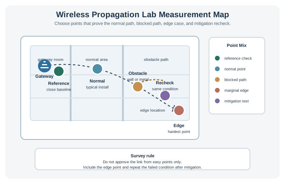
Run it: Use the range estimator below to place your edge point on evidence instead of convenience. Set the Radio Type and Environment to match this deployment, then read the Range Field and Budget Pressure to see how far this radio should reach and where the link runs out of margin. Use Radio Comparison and Technology Fit to check whether your farthest planned device location is realistic, then put the edge and obstacle points at the distances the estimate calls marginal rather than at easy places to stand.
Use this point mix:
- Reference point: close, stable, and repeatable; confirms the radio is configured correctly.
- Normal point: typical installation location; checks expected day-to-day behavior.
- Obstacle point: wall, door, vehicle, cabinet, rack, or enclosure in the path.
- Edge point: farthest or most difficult planned device location.
- Remeasure point: the location where the mitigation will be retested.
29.17 Avoid Best-Case Surveys
A map made from only easy points will approve a weak design. Include corners, low mounting heights, closed doors, metal, crowded rooms, and busy operating periods when those conditions are part of the real deployment.
29.18 Lab 3: Quality Diagnosis
A single RSSI value is not enough. Pair signal strength with SNR and delivery behavior.
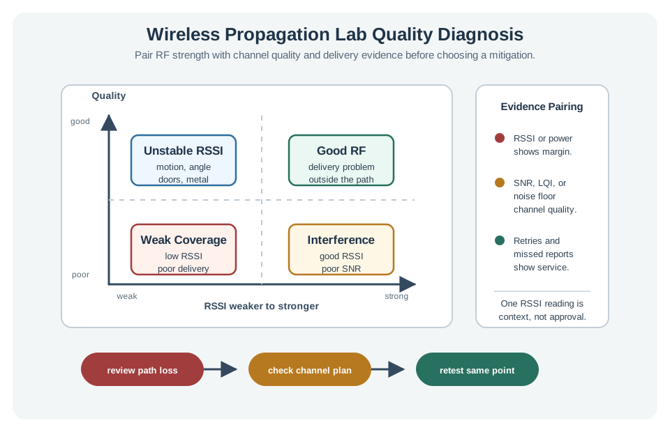
29.18.1 Weak RSSI and Poor Delivery
Review path loss, antenna placement, mounting height, obstruction, gateway location, and receiver mode.
29.18.2 Good RSSI and Poor SNR
Review interference, co-channel use, nearby transmitters, receiver overload, and channel plan.
29.18.3 Unstable RSSI
Review multipath, motion, orientation, doors, vehicles, people, and time-varying shadowing.
29.18.4 Good RF, Poor Delivery
Review firmware timing, queues, credentials, radio scheduling, payload size, gateway load, and backend delivery.
29.19 Lab 4: Mitigation Test
Choose one mitigation that matches the diagnosis, then remeasure the same point.
Common mitigation choices:
- Move the receiver, gateway, or antenna to improve the path.
- Change antenna orientation or mounting height.
- Reduce obstruction from enclosures, metal, body placement, or cable routing.
- Change channel or band when SNR and occupancy evidence point to coexistence.
- Add another gateway or receiver when the edge point cannot be made robust.
- Change reporting interval, retry policy, packet size, or data rate when protocol behavior is part of the failure.
Do not change three variables at once. If placement, channel, and packet size all change together, the review record cannot explain which change fixed the link.
29.20 Lab 5: Release Record
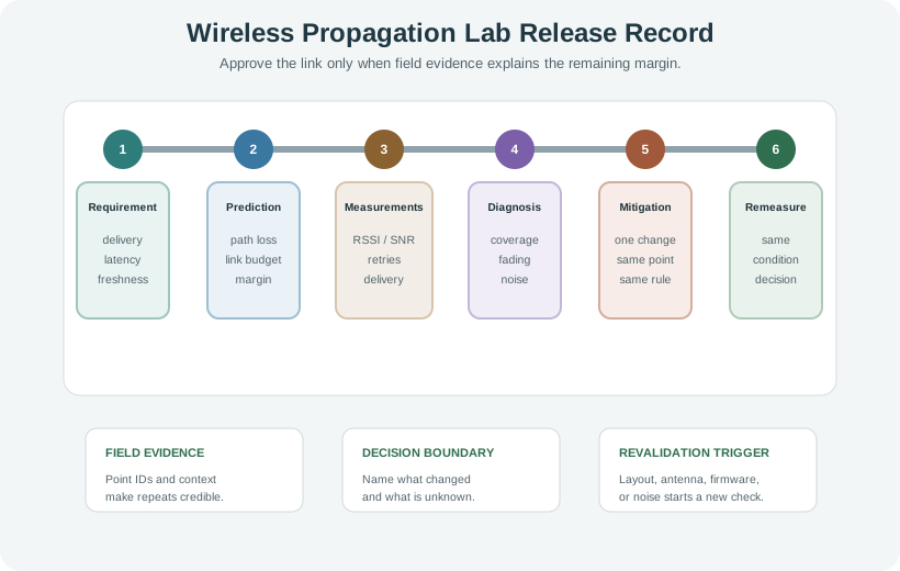
A release record should include:
- The application requirement: delivery, latency, freshness, and availability.
- The radio configuration: band, channel, data rate, packet size, antenna, power setting, and receiver mode.
- The prediction: link-budget terms and expected reserved margin.
- The measurement set: point IDs, RSSI, SNR, retries, packet delivery, and context.
- The diagnosis: weak coverage, fading, interference, placement, or non-RF behavior.
- The mitigation and recheck: what changed, where it was remeasured, and whether it now meets the requirement.
- The revalidation trigger: layout change, antenna change, firmware mode change, gateway move, new interference source, or new installation area.
29.21 Check Your Understanding
Release Record Label Check
Evidence Matching
Lab Order
Knowledge Check
29.22 Common Pitfalls
29.22.1 Measuring Only the Best Reading
Wireless links fluctuate. Record minimum, median, and delivery behavior over several samples instead of approving the strongest number you saw.
29.22.2 Treating RSSI as the Whole Story
RSSI says the receiver sees energy. It does not prove clean SNR, low retries, correct credentials, healthy queues, or successful backend delivery.
29.22.3 Testing the Wrong Mounting Condition
A device on a desk, in a hand, inside an enclosure, behind metal, or mounted near the floor can produce different measurements. Test the actual installation geometry.
29.22.4 Remeasuring After Changing the Scenario
If the failure happened during peak occupancy or equipment activity, the fix must be remeasured during that same condition.
29.23 Try It: Link Budget and Fresnel Explorer
Use the inline RF planning widget to compare the lab’s distance, frequency, antenna, system-loss, receiver-sensitivity, and obstacle assumptions before you collect field measurements.
29.24 Preserve Causality and Margin
A release-ready propagation lab starts with the acceptance target, not with the radio. Write the minimum delivery rate, maximum report age, latency expectation, availability need, and installation boundary before collecting data. Then freeze the configuration: band, channel, data rate or spreading factor, transmit power, antenna, packet size, reporting interval, firmware mode, gateway or access-point identity, receiver sensitivity assumption, and any duty-cycle or listen-before-talk constraint that affects airtime. Missing configuration notes are hard to reconstruct after a field walk.
Keep the evidence at the granularity used for the design decision. For a Wi-Fi or BLE prototype, the sheet may need RSSI samples, packet delivery, channel, location, and antenna orientation. For LoRaWAN, keep gateway RSSI, packet SNR, spreading factor, data rate, gateway ID, frame-counter evidence, and time-of-day context from a network server such as ChirpStack or The Things Stack. For IEEE 802.15.4, keep LQI or equivalent link-quality evidence when the platform exposes it, plus retries, acknowledgments, channel, and sniffer notes from tools such as Wireshark with an 802.15.4 capture interface.
29.24.1 Protocol-Specific Evidence
| Radio family | Evidence that keeps the result repeatable | Common stale-evidence trigger |
|---|---|---|
| Wi-Fi | RSSI, channel, data rate, retry behavior, access-point identity, noise or utilization when available | Access-point move, channel plan change, rate policy change, or new nearby traffic |
| BLE | RSSI samples, advertising or connection interval, transmit power, orientation, phone/gateway model, packet loss or reconnect events | Enclosure change, body placement, firmware timing change, or gateway model change |
| LoRaWAN | Gateway RSSI, packet SNR, spreading factor, data rate, gateway ID, frame counter, receive-window behavior | Spreading-factor change, gateway move, antenna change, duty-cycle pressure, or new installation area |
| IEEE 802.15.4 | LQI or equivalent quality metric, channel, acknowledgments, retries, sniffer notes, mesh parent when applicable | Channel change, mesh topology change, enclosure change, or new co-channel traffic |
Most propagation-lab mistakes come from treating one RSSI value as a stable property of a location. RSSI is receiver-specific, often averaged by firmware, and affected by antenna orientation, polarization, channel bandwidth, modulation, coding, receiver gain state, multipath, and nearby bodies or metal. Two radios can report different RSSI for the same packet, and some systems expose link quality, SNR, or retry counters more reliably than a calibrated power reading. That is why the release record keeps configuration and delivery evidence beside the RF number.
The path-loss model is still useful, but it is a planning model. A common form is:
\[ PL(d) = PL(d_0) + 10n\log_{10}(d/d_0) + X \]
Here, n is the environment exponent and X represents shadowing and measurement variation. The measurement set estimates whether the remaining fade margin survives realistic variation. A link with only 1 or 2 dB of apparent margin in a quiet hallway is not equivalent to a link with 12 dB of margin measured at the edge point during normal operation.
29.24.2 Diagnose Before You Fix
Classify the result before choosing a mitigation. Low RSSI with poor delivery points toward path loss, antenna placement, receiver mode, or gateway location. Good RSSI with poor SNR or high retries points toward interference, receiver overload, channel occupancy, or coexistence. Large RSSI swings after small movement point toward multipath, body blocking, orientation, or shadowing. Good RF metrics with missed reports shifts the investigation toward MAC retries, firmware queues, payload size, credentials, gateway backhaul, broker behavior, or backend ingestion.
Interference adds another layer because high received energy can be harmful. A receiver may report strong RSSI while SNR, packet delivery, or retries degrade because the wanted signal is mixed with co-channel traffic, adjacent-channel energy, impulsive noise, or receiver front-end overload. In that case, increasing transmit power may be ineffective or even harmful. The better evidence is a time-correlated record: channel, SNR or noise-floor estimate, retry burst, packet loss, nearby transmitter activity, and whether the symptom disappears on a quieter channel or at another time.
When you test a mitigation, change one variable and rerun the original failing point. If a channel change fixed a busy-period coexistence problem, remeasure during the busy period. If a new antenna orientation fixed a metal-cabinet shadow, remeasure with the cabinet closed and the device mounted as deployed. The release note should name the chosen mitigation, the rejected alternatives, and the revalidation trigger that would make the evidence stale.
29.25 Summary
A wireless propagation lab is a release workflow, not a demo. Start with a link-budget prediction, then measure real points with RSSI, SNR, retries, packet delivery, location, obstacle, orientation, and time context. Diagnose the gap before changing the design, apply one mitigation at a time, and remeasure the original failure condition. The final artifact is a release record that explains why the link is acceptable, where it remains risky, and what change will require revalidation.
29.26 What’s Next
29.26.1 Radio Wave Basics for IoT
Review frequency, wavelength, antenna behavior, and dBm notation.
29.26.2 Fading and RF Interference
Separate fading, weak coverage, and coexistence symptoms.
29.26.3 Path Loss and Link Budgets
Connect this lab’s measurements back to prediction and margin.
29.27 Key Takeaway
A propagation lab turns assumptions into measurements. Compare predicted and observed RSSI, packet loss, distance, antenna orientation, obstruction, and interference before trusting a deployment plan.