flowchart TD
    A[Deployment requirement] --> B{Needs local timing or offline control?}
    B -- yes --> C[Place control near device or edge]
    B -- no --> D{Is raw data too large for backhaul?}
    D -- yes --> E[Filter or aggregate at gateway]
    D -- no --> F{Needs fleet-wide analytics?}
    F -- yes --> G[Store and analyze in cloud]
    F -- no --> H[Use the simplest direct path]
    C --> I[Record validation test]
    E --> I
    G --> I
    H --> I
36 IoT Architecture Planner
Interactive Tool for Designing End-to-End IoT Systems
fundamentals
planner
36.1 In 60 Seconds
An IoT architecture spans five layers – sensing, networking, processing, cloud, and application. This interactive planner helps you design a complete system by selecting components at each layer, estimating data volumes and costs, and matching your choices to proven architecture patterns.
36.2 Start With the Story
Start with a product meeting where someone says just use the protocol we know, while the deployment quietly needs different range, power, latency, security, and operations evidence. The core idea in IoT Architecture Planner is simple: protocol choice is a constraint problem, not a popularity contest, and the defensible answer comes from eliminating bad fits before scoring good candidates. This page focuses that idea on Plan and visualize your IoT architecture including sensors, edge processing, connectivity, cloud services, and data flow. In everyday IoT, parking sensors, wearables, logistics tags, and building retrofits need different proof even when they all send small messages. Start simple: state the hard constraints, reject impossible options, compare the finalists, and then validate the chosen protocol in the field.
36.3 Chapter Scope
This chapter focuses on end-to-end architecture decision-making.
- Use Protocol Selector Wizard for protocol-only decisions.
- Use Simulation Catalog for broad simulator/tool discovery.
- Use this chapter when integrating sensing, connectivity, processing, cloud, and application choices as one design.
Chapter Roadmap
Use the planner in four passes:
- First frame the job: application, scale, criticality, and the five responsibility layers.
- Then size the sensing and network choices so 500 sensors, 50 hectares, gateway count, and battery life become explicit constraints.
- Next move into processing, cloud, application interfaces, cost, and recommendation logic.
- Finally use the quizzes, deep dive, and summary to turn the selected architecture into a validation record.
Checkpoints recap the evidence; the existing physics panel and interactives remain companion material.
Phoebe’s Field Notes: Where a “5-Year Battery Life” Requirement Comes From

Phoebe’s Why
“Five-year battery life” is not a firmware setting – it is a chemistry and arithmetic claim. A cell’s milliamp-hour rating only becomes an energy budget once terminal voltage multiplies in, and that budget bleeds away on its own through self-discharge long before the radio spends a single joule. For a sensor waking a few times a day, the years-long sleep current and the cell’s own leakage usually cost more than the brief transmit bursts do – which is exactly why the vineyard scenario’s chemistry choice matters as much as its duty cycle. The soil sensor itself is a second physics story: a capacitive probe reads volumetric water content because water’s relative permittivity is roughly twenty times that of dry soil, so soil capacitance is dominated by how much water sits between the plates.
The Derivation
Charge rating becomes an energy budget only once voltage multiplies in:
\[E_{cell}\,\mathrm{(Wh)} = C\,\mathrm{(Ah)} \times V\]
Current through internal resistance sags the terminal voltage under load:
\[V_{terminal} = V_{oc} - I R_{int}\]
Usable energy after self-discharge over time \(t\) and a derating margin \(\delta\):
\[E_{usable} = E_{cell}\,(1-k)^{t}\,(1-\delta)\]
The soil probe’s governing equation – a parallel-plate capacitor, dominated by soil permittivity \(\varepsilon_r\):
\[C = \frac{\varepsilon_0\,\varepsilon_r\,A}{d}\]
Worked Numbers: The Vineyard Sensor’s 5-Year Budget
The chapter fixes 500 sensors, 5 readings/day, and a 5-year battery-life requirement but not a cell, so take a standard choice for that exact duty cycle: one ER14505-class Li-SOCl\(_2\) AA cell (\(C = 2.4\) Ah, \(V = 3.6\) V, self-discharge \(\approx 1\)%/year).
- \(E_{cell} = 2.4 \times 3.6 = 8.64\) Wh
- Over 5 years: self-discharge factor \((0.99)^{5} = 0.951\); with a 10% derating margin, \(E_{usable} = 8.64 \times 0.951 \times 0.90 = 7.39\) Wh
- Sleep cost dominates: at a \(3\ \mu\mathrm{A}\) sleep current, \(E_{sleep} = 3\times10^{-6} \times 3.6 \times (5\times365\times24\times3600) = 1{,}703\) J \(= 0.473\) Wh over 5 years
- Active cost is small by comparison: at \(9{,}125\) readings (\(5/\mathrm{day} \times 1825\) days) drawing 40 mA for 0.2 s each, \(E_{active} = 9{,}125 \times 0.040 \times 3.6 \times 0.2 = 263\) J \(= 0.0730\) Wh
- Total spent \(\approx 0.546\) Wh against a \(7.39\) Wh usable budget – only about 7.4%, leaving generous margin for the low-temperature capacity fade and radio retries this estimate does not model
- Voltage sag: Li-SOCl\(_2\)’s internal resistance (\(R_{int} \approx 10\ \Omega\)) against the 40 mA active burst sags the terminal by \(0.040 \times 10 = 0.4\) V – from 3.6 V to 3.2 V, a real dip worth checking against the radio’s brown-out threshold
36.4 IoT Architecture Planner
Learning Objectives
By using this interactive tool, you will be able to:
- Design a complete five-layer IoT architecture from sensing through application delivery
- Evaluate edge-versus-cloud processing trade-offs for a given latency and bandwidth budget
- Estimate hardware and recurring costs for different architectural approaches
- Diagnose potential bottlenecks in data flow, gateway capacity, and processing pipelines
- Select an architecture pattern (direct-to-cloud, gateway-based, or edge-heavy) that matches deployment constraints
- Justify component choices by linking sensor count, data volume, and cost projections to business requirements
Treat the planner as a decision record, not just a calculator: each slider should expose one assumption to prove before scale.
36.5 How It Works: Turn Requirements Into An Architecture
Use the planner as a requirements-to-evidence loop.
- Name the deployment job. Start with the environment, users, sensing task, latency target, data volume, and maintenance constraints.
- Place each layer. Decide what belongs in sensing, connectivity, edge/gateway, cloud, and application layers.
- Quantify the stress points. Estimate message rate, payload size, gateway load, storage, recurring cost, and response-time pressure.
- Choose the pattern. Select direct-to-cloud, gateway-based, or edge-heavy architecture only after the weak layer is visible.
36.6 Incremental Examples
Beginner Example: A single greenhouse sensor can send periodic readings directly to a cloud dashboard if latency is low-risk and connectivity is reliable.
Intermediate Example: A building with many rooms may need a gateway to reduce traffic, normalize protocols, and keep some control local.
Advanced Example: A safety-critical industrial line may need edge processing, buffered data, local failover, and a cloud layer for fleet analytics rather than real-time control.
36.7 Quick Checks
Checkpoint: Architecture Frame
You now know:
- The planner is for end-to-end architecture decisions, while the Protocol Selector Wizard is for protocol-only choices.
- A complete design must place sensing, networking, processing, cloud, and application responsibilities.
- The first evidence loop is simple: name the deployment job, place each layer, quantify stress points, then choose the pattern.
36.8 Try It Yourself
Write a five-layer architecture note for one IoT scenario. For each layer, list one chosen component, one assumption, and one validation task.
36.9 See Also
- Protocol Selector Wizard - narrows the connectivity choice inside the architecture.
- Sensor-to-Network Pipeline - traces evidence from sensing through transport.
- Application Domains Overview - helps anchor the architecture to a real application need.
36.10 Key Concepts
- Architecture layer: One responsibility band in the system, such as sensing, network, processing, cloud, or application.
- Placement decision: The choice of whether a function runs on a device, gateway, edge server, or cloud service.
- Data-volume estimate: A first-order calculation that turns sensor count, frequency, and payload size into bandwidth and storage pressure.
- Gateway capacity: The practical limit on how many devices, messages, protocol conversions, and local tasks one gateway can handle.
- Architecture pattern: A repeatable shape such as direct-to-cloud, gateway-centric, edge-heavy, mesh, or high-availability.
- Validation task: A specific measurement, pilot, failure drill, or simulation used to prove the architecture’s riskiest assumption.
36.10.1 Key Takeaway
In one sentence: A well-designed IoT architecture balances sensing needs, connectivity options, processing location, and cost constraints across five interconnected layers.
Remember this rule: Process data at the edge when latency matters, send to cloud when you need scale - your architecture should optimize the edge/cloud split for your specific requirements.
No-One-Left-Behind Architecture Loop
- Start with a clear deployment scenario and constraints.
- Decide one layer at a time, validating dependencies.
- Quantify data volume, latency, and cost before finalizing.
- Reinforce by testing assumptions with one simulation or lab.
36.11 Prerequisites
Before using this planner, review:
- IoT Reference Models: Understanding of IoT architecture layers
- Edge-Fog Computing: Edge vs. cloud processing concepts
- Protocol Selector Wizard: Choose connectivity before designing architecture
For Beginners: IoT Architecture = Blueprint for Your System
Simple Analogy: Building a House
Designing IoT architecture is like planning a house:
| House Component | IoT Equivalent | Purpose |
|---|---|---|
| Sensors (smoke, motion) | IoT Sensors | Detect what’s happening |
| Wiring | Network/Protocols | Connect everything |
| Electrical panel | Gateway/Edge | Process locally |
| Utility connection | Cloud Services | Connect to outside world |
| Smart home app | Dashboard/App | Control and monitor |
Three Architecture Patterns:
- Direct-to-Cloud: Sensors → Cloud (simple, but needs internet)
- Gateway-Based: Sensors → Gateway → Cloud (most common)
- Edge-Heavy: Sensors → Edge Processing → Cloud (smart, less data)
36.12 Step 1: Define Your Application
Next comes scale: do not pick gateways, cloud tiers, or edge processing until deployment size and message rate have numbers attached.
Worked Example: Architecture Planning for Smart Agriculture
Scenario: A vineyard owner wants to monitor 50 hectares (500 sensors: soil moisture, temperature, humidity) to optimize irrigation.
Step-by-step planning:
- Define scope: 500 sensors across 50 hectares, cellular connectivity (no Wi-Fi), 5-year battery life required
- Calculate data volume: 500 sensors × 5 readings/day × 20 bytes/reading = 50 KB/day = 1.5 MB/month
- Estimate costs: Sensors ($15 each = $7,500) + gateways ($200 each, need 10 = $2,000) + cellular ($2/month per gateway) = $9,500 upfront + $240/year
- Choose architecture: Gateway-based with LoRaWAN (long range, low power) + 4G backhaul, 50% edge processing (local alerts for irrigation triggers)
Outcome: System paid for itself in year 1 through 30% water savings ($12,000/year).
Putting Numbers to It
Architecture choices should be grounded in data-volume math before selecting gateways, cloud plans, and retention policies:
\[ D_{\text{month}} = \frac{N_{\text{sensors}} \times f_{\text{day}} \times B_{\text{msg}} \times 30}{1024^2} \text{ MB} \]
where \(D_{\text{month}}\) is monthly data volume in MB, \(N_{\text{sensors}}\) is sensor count, \(f_{\text{day}}\) is messages per sensor per day, and \(B_{\text{msg}}\) is bytes per message.
Worked example: With 500 sensors sending every 15 minutes (\(f_{\text{day}}=96\)) and 32-byte payloads:
\[ D_{\text{month}} = \frac{500 \times 96 \times 32 \times 30}{1024^2} \approx 43.95 \text{ MB/month} \]
If edge filtering removes 70% of non-actionable records, cloud ingest becomes about \(13.2\) MB/month. That reduction directly affects backhaul usage, storage cost, and query latency.
Common Mistake: Underestimating Gateway Count
Problem: Assuming one gateway can cover an entire deployment area.
Reality: LoRaWAN range is heavily affected by terrain and obstacles. A single gateway might reach 2-5 km in open fields, but only 500m in dense agriculture with trees/hills.
Fix: Use radio propagation tools (e.g., RadioMobile) to model actual coverage before ordering hardware. Budget 1 gateway per 20-50 sensors in challenging terrain.
36.13 Step 2: Sensing Layer
Layer 1: Sensors and Actuators
The perception layer captures physical world data and executes actions.
36.14 Step 3: Network Layer
Layer 2: Connectivity
How sensors connect and communicate data.
Decision Framework: Choosing Connectivity Protocol
Use this table to select the right protocol based on your constraints:
| Your Constraint | Choose | Why |
|---|---|---|
| Indoor deployment, power available | Wi-Fi | Highest bandwidth, existing infrastructure |
| Indoor sensors, battery powered | Bluetooth LE or Zigbee | Low power, good indoor range (10-30m) |
| Outdoor, sensors spread 1-5 km | LoRaWAN | Long range, very low power, proven for agriculture |
| Mobile assets (vehicles, containers) | Cellular (NB-IoT/LTE-M) | Ubiquitous coverage, higher cost |
| Urban dense deployment | Thread or Zigbee | Mesh networking handles interference |
| 10+ year battery life | LoRaWAN or Sigfox | Ultra-low power modes, infrequent transmission |
Real numbers example: 100 soil sensors, 5 readings/day for 5 years - LoRaWAN: 2× AA batteries last 5-7 years, data cost ~$50/year (gateway backhaul) - Cellular NB-IoT: Battery life 2-3 years, data cost ~$200/year (per-device SIM) - Wi-Fi: Must plug in, data cost $0 (local network)
36.14.1 Quick Knowledge Check: Gateway Architecture
Before proceeding, test your understanding of the gateway decisions you just made.
Checkpoint: Scale and Connectivity
You now know:
- The vineyard example binds the decision to 500 sensors, 50 hectares, 5 readings/day, 20 bytes/reading, 50 KB/day, and 1.5 MB/month.
- Gateway count is not a guess: the chapter warns that dense agriculture may need one gateway per 20-50 sensors rather than one gateway for the whole area.
- The network must follow the constraint: LoRaWAN fits wide, low-rate field sensing; Bluetooth mesh or Wi-Fi extenders create power and coverage problems.
36.15 Step 4: Processing Layer
Once connectivity is plausible, look for the next bottleneck: where the data should be reduced, buffered, or acted on before it reaches the cloud.
Layer 3: Where to Process Data
Decide between edge, fog, and cloud processing.
36.16 Step 5: Application Layer
Layer 4: Business Applications
End-user applications and integrations.
Checkpoint: Processing Placement
You now know:
- Processing location follows the bottleneck: latency, resilience, privacy, and bandwidth can justify edge-heavy design.
- Raw vibration data at 500 sensors, 1 kHz, and 4 bytes/sample becomes 16 Mbps, which cannot fit a 2 Mbps cellular backhaul.
- Edge processing is valuable only when it changes the evidence: filtering, FFT, anomaly detection, downsampling, buffering, or local control must reduce risk, not just add another layer.
36.17 Architecture Visualization
36.18 Cost Estimation
36.19 Architecture Recommendations
36.20 Architecture Patterns
Based on your selections, here are relevant architecture patterns:
Recommended Patterns for Your Application
36.21 Your Configuration Summary
After visualization and recommendations, pause before treating the output as final. The summary below is a candidate architecture to validate.
36.22 Common Pitfalls
1. Prioritizing Theory Over Measurement
Relying on theoretical models without profiling actual behavior leads to designs that miss performance targets by 2-10×. Always measure the dominant bottleneck in your specific deployment environment — hardware variability, interference, and load patterns routinely differ from textbook assumptions.
2. Ignoring System-Level Trade-offs
Optimizing one parameter in isolation (latency, throughput, energy) without considering impact on others creates systems that excel on benchmarks but fail in production. Document the top three trade-offs before finalizing any design decision and verify with realistic workloads.
3. Skipping Failure Mode Analysis
Most field failures come from edge cases that work in the lab: intermittent connectivity, partial node failure, clock drift, and buffer overflow under peak load. Explicitly design and test failure handling before deployment — retrofitting error recovery after deployment costs 5-10× more than building it in.
36.23 What’s Next
- Select protocols: Protocol Selector Wizard to refine connectivity choices based on your architecture constraints.
- Plan your learning: Learning Paths to create a curriculum matched to your design goals.
- Explore simulations: Simulation Playground to test your architecture virtually before committing to hardware.
- Build a prototype: Capstone Projects to apply your architecture in a guided end-to-end project.
- Deepen reference models: IoT Reference Models to compare your design against standard IoT architecture frameworks.
- Reinforce decisions: IoT Games Hub to practise architecture trade-off reasoning through challenge rounds.
36.25 Concept Relationships
IoT Architecture Planning Builds on: system design principles and layer models. Leads to: platform selection and protocol choice. Contrasts with: ad-hoc device deployment.
Edge vs Cloud Processing Builds on: computing fundamentals and latency requirements. Leads to: edge computing frameworks and fog architectures. Contrasts with: pure cloud-only architectures.
Gateway Architecture Builds on: protocol translation and network layers. Leads to: mesh networking and multi-protocol gateways. Contrasts with: direct device-to-cloud approaches.
Cost Estimation Builds on: TCO analysis and subscription models. Leads to: vendor negotiation and ROI calculation. Contrasts with: one-time hardware cost focus.
Redundancy Planning Builds on: system reliability and fault tolerance. Leads to: high-availability architectures and disaster recovery. Contrasts with: single-point-of-failure designs.
See Also
Related Interactive Tools:
- Protocol Selector Wizard - Choose connectivity protocols based on your architecture constraints
- Learning Paths - Get personalized curriculum recommendations for system design
- IoT Games Hub - Reinforce architecture trade-off decisions through challenge rounds
Architecture Deep Dives:
- IoT Reference Models - Standard architecture frameworks and patterns
- Edge-Fog Computing - When to process at edge vs cloud
- Integration Gateways - Protocol translation and aggregation patterns
Cost and Business Planning:
- IoT Business Models - Monetization and revenue strategies
- Simulation Catalog - Find calculators and planning tools
Implementation Guides:
- Capstone Projects - Build complete end-to-end systems
- Simulation Playground - Test architectures virtually
36.26 Check Your Understanding
36.26.1 Match Architecture Layers to Their Primary Responsibility
36.26.2 Order: IoT Architecture Design Process
36.26.3 Label the Diagram
36.27 Practice the Architecture Record
36.27.1 Code Challenge
36.27.2 Order the Steps
Checkpoint: Architecture Record
You now know:
- Cost estimates combine hardware, cloud services, and connectivity; the chapter’s edge-filtering example moves 43.95 MB/month toward about 13.2 MB/month after 70% filtering.
- Recommendations are warnings to test, not automatic approvals.
- A complete architecture record names components, assumptions, data flow, security measures, and validation tasks in order.
36.27.3 Match the Concepts
36.28 Deep Dive: Place Computation Where the Constraint Lives
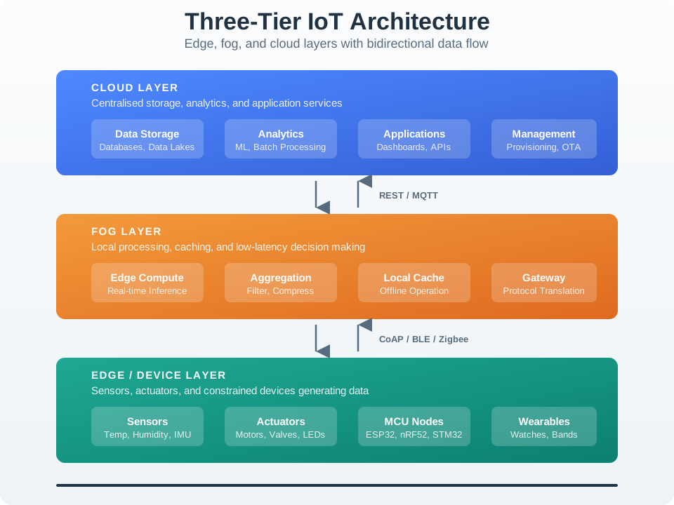
An IoT architecture spans sensing, networking, processing, cloud, and application layers, but the decision that shapes cost and behavior most is where computation runs. The same analytics can execute on the device, at the edge through a nearby gateway, or in the cloud. Each placement trades a different set of properties.
Push work toward the device and you gain low latency, offline autonomy, and privacy, but you are limited by compute and battery. Push it to the cloud and you gain large-scale storage, analytics, and fleet-wide visibility, but you pay in latency, bandwidth, connectivity dependence, and exposure of raw data. The edge sits between those extremes.
36.28.1 Compare the Three Tiers
| Property | On-device | Edge / gateway | Cloud |
|---|---|---|---|
| Latency | Lowest, often milliseconds | Low on the local network | Highest because of the internet round trip |
| Compute and storage | Very limited | Moderate | Effectively elastic |
| WAN bandwidth | Minimal when only results leave the device | Reduced by aggregation | Highest when raw data is uploaded |
| Privacy | Data can stay local | Data can stay on-site | Raw or detailed data may leave the premises |
| Offline operation | Can keep working | Can keep the site working | Depends on connectivity |
A supermarket cold-room monitor shows the split. It may read DS18B20 or SHT31 probes every few seconds, trigger a local buzzer when temperature crosses a food-safety threshold, and publish summaries to a cloud dashboard. The alarm decision belongs on the device or gateway because staff need it during an internet outage. The hourly trend, cross-site comparison, and maintenance report can live in the cloud because they need storage and fleet context more than millisecond timing.
Video analytics creates the same pressure. Streaming raw 1080p video to the cloud for hazard detection costs large amounts of bandwidth, adds latency, and ships sensitive footage off-site. Running the detection model on a gateway or camera means only a compact event travels upstream: timestamp, camera ID, confidence score, and a short retained clip when policy allows. The cloud still aggregates events and retrains models, but it should not sit in the real-time inference path.
36.28.2 Hybrid Systems Need State Ownership
The device-vs-edge-vs-cloud choice is rarely all-or-nothing. Strong architectures are hybrids that place each function where it fits: filter and threshold on the device, aggregate and run time-critical logic at the edge, then store, analyze across sites, and train models in the cloud. Data gets smaller and less time-sensitive as it moves up the tiers.
A building HVAC system can run its per-room control loop on local controllers so comfort continues during WAN loss, have the site gateway aggregate zone data and enforce schedules, and send hourly summaries to the cloud for cross-building optimization and fault prediction. Each tier does the job it is suited for, and the architecture degrades gracefully instead of failing when the cloud link drops.
The hidden mechanism is ownership of state. The room controller owns immediate actuator state, the gateway owns site schedule and buffered telemetry, and the cloud owns fleet models and reporting history. Each handoff should name message schema, retry behavior, timestamp source, and stale-data rules. Without that ownership map, a hybrid design can become three partial systems that disagree during an outage.
Validate the placement by forcing failures: disconnect WAN, restart the gateway, replay delayed messages, and confirm the room controller still follows local limits while the cloud marks the site data as stale.
36.29 Summary
The IoT Architecture Planner helps you design complete IoT systems:
- 5-layer design covering sensing, network, processing, cloud, and application
- Data volume estimation based on sensors, frequency, and message size
- Cost projection for hardware and ongoing services
- Edge vs. cloud trade-offs with automatic recommendations
- Pattern matching to relevant architecture approaches
Key Architecture Principles
- Start small, scale up - Begin with proven patterns, add complexity as needed
- Design for failure - Assume components will fail; build redundancy
- Secure by design - Security is not an afterthought
- Optimize data flow - Process at the edge when possible to reduce costs
- Plan for evolution - Requirements change; choose flexible architectures
For Kids: Meet the Sensor Squad!
Sammy the Sensor is excited! “I want to build the BIGGEST IoT system ever!” he shouts.
Max the Microcontroller laughs. “Whoa, slow down! Building a great IoT system is like planning an awesome school project. You need a plan!”
“First,” says Lila the LED, “you pick what you want to SENSE – like temperature, motion, or light. That’s the sensing layer!”
“Then,” adds Max, “you figure out HOW to send your data. Wi-Fi? Bluetooth? LoRa? That’s the network layer!”
Bella the Battery pipes up: “And don’t forget about me! If you process data close to the sensors (at the ‘edge’), I last longer because you don’t have to send everything far away to the cloud!”
“So an IoT architecture is like a relay race,” Sammy says. “Sensors collect data, the network passes it along, the processor does something smart with it, the cloud stores it, and the app shows it to people!”
“Exactly!” cheers the whole Squad. “Layers working together – that’s architecture!”
Fun fact: The biggest IoT systems in the world (like smart cities) have MILLIONS of sensors all working together through these five layers!