10 Choosing an IoT Data Format
Choosing How Sensor Readings Are Encoded for the Link You Have
10.1 In 60 Seconds
Choose the most readable data format that still fits the link. JSON is a good default when bandwidth and power are comfortable, CBOR or MessagePack help when a compact self-describing payload is needed, Protocol Buffers fit stable schema contracts, and custom binary belongs only on links where every byte is worth the decoder discipline.

Phoebe’s Why
A radio wave’s power does not vanish over distance – it spreads. Send a fixed amount of power from an antenna and by the time it has travelled distance \(d\), that power is smeared over the surface of a sphere of radius \(d\), so the density any receiver sees falls as \(1/d^2\). Double the distance and the same power covers four times the area, so every square metre gets a quarter as much – the inverse-square law behind Friis’s free-space loss. Real ground paths are worse than free space: reflections, canopy, and terrain roughness make the loss climb faster than \(1/d^2\), so engineers replace the exponent 2 with a measured path-loss exponent \(n\). A vineyard soil node fights that steeper loss with LoRa’s slowest, most robust setting, SF12, which trades data rate for extra processing gain. That trade is also why the payload has to be small: the long symbol time bought for sensitivity leaves less airtime per duty-cycle window, and airtime is metered by both regulation and battery.
The Derivation
Free-space loss at a short reference distance \(d_0\):
\[\mathrm{FSPL}_{\mathrm{dB}}(d_0) = 20\log_{10}\!\left(\frac{4\pi d_0}{\lambda}\right)\]
Log-distance model beyond \(d_0\), with path-loss exponent \(n\):
\[PL(d) = \mathrm{FSPL}_{\mathrm{dB}}(d_0) + 10\,n\,\log_{10}\!\left(\frac{d}{d_0}\right)\]
Fade margin at the receiver:
\[M = \mathrm{EIRP} - PL(d) - S\]
where \(S\) is receiver sensitivity. The link holds only while \(M \geq 0\).
Worked Numbers: The Vineyard Link
- Wavelength at 868 MHz: \(\lambda = 3.00\times10^{8}/868\times10^{6}\) \(= 0.346\) m
- FSPL at \(d_0=1\) m: \(20\log_{10}(4\pi(1)/0.346)\) \(= 20\log_{10}(36.4)\) \(= 31.2\) dB
- Path loss to 3 km, rural \(n=2.7\) (catalog-typical exponent): \(31.2 + 10(2.7)\log_{10}(3000)\) \(= 31.2 + 93.9\) \(= 125\) dB
- Received power at 14 dBm EIRP (EU868 sub-band limit): \(14 - 125 = -111\) dBm
- Margin: SF12 sensitivity \(-137\) dBm (catalog) gives \(-111-(-137) = 25.9\) dB; SF7 sensitivity \(-123\) dBm gives only \(11.9\) dB
- Add 15 dB vine-canopy/terrain loss (catalog-typical foliage attenuation): SF12 keeps \(10.9\) dB margin; SF7 goes to \(-3.1\) dB and drops the link – this is why the node must run SF12, capping the payload near 51 bytes at \(\approx 250\) bit/s
- Battery tie, at the chapter’s own 44 mA radio current: CBOR’s 1.5 s airtime costs \(44\times1.5 = 66.0\) mA\(\cdot\)s \(= 18.3\) \(\mu\)Ah; the 8-byte binary layout’s 0.26 s airtime costs \(44\times0.26=11.4\) mA\(\cdot\)s \(=3.18\) \(\mu\)Ah – a \(18.3/3.18 = 5.75\times\) saving, matching the chapter’s “roughly five to six times” claim from first principles
10.2 Start With the Story
Start with a message crossing a link where the receiver must know where the packet starts, what each field means, and whether any byte was corrupted. The core idea in Choosing an IoT Data Format is simple: packet and format design is about boundaries, field meaning, compactness, checks, and the evidence that the receiver can parse the payload safely. This page focuses that idea on Guide to IoT data-format choices across JSON, CBOR, Protocol Buffers, and custom binary, with payload sizing and schema-evolution trade-offs. In everyday IoT, JSON, CBOR, Protobuf, custom binary, framing bytes, CRCs, and overhead budgets are practical choices with reliability and debugging costs. Start simple: draw the packet as fields, mark the payload and checks, then justify the format only after the parse path is clear.
10.3 Match Format to Link Budget
A data format is the language a device uses to write down a reading before it leaves the chip. The same temperature value can be sent as the text {“temp”:23.5} or as a few packed bytes. Both carry the measurement, but they cost very different amounts of bandwidth, radio time, and battery.
The important idea is not “make every message as small as possible.” The important idea is fit: the format should be the most readable one that still fits the link you actually have.
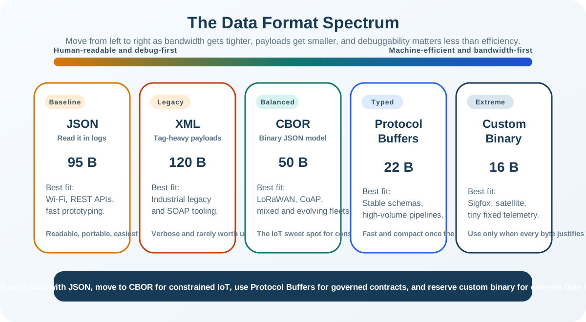
The core rule is practical: pick the most human-readable format your link can afford. Use text such as JSON when bandwidth is comfortable, step down to a compact binary format when the radio payload is tight, and reserve hand-packed binary for the most constrained links.
Think of packing a suitcase. Labelling every item (“blue shirt”, “toothbrush”) is easy to unpack later but wastes space; that is JSON. Vacuum-sealing with short labels saves room while staying organized; that is a compact binary format such as CBOR. Compressing everything into the smallest possible bundle is the most efficient but you must remember exactly where each item went; that is custom binary.
A real format choice starts with the device’s link, not the developer’s preference. A smart-parking sensor on NB-IoT may have enough room for a readable JSON message because the payload limit is measured in hundreds of bytes. A soil probe on LoRaWAN at a low data rate may need CBOR or integer scaling because the available payload is much smaller. A Sigfox tracker with a roughly 12-byte uplink may force a hand-packed layout with a version byte, bit flags, and scaled integers. The same reading can therefore move across the spectrum as the radio, battery, and debugging needs change.
The One-Minute Format Decision
Size the link first
Start with the real constraint: the maximum payload, the data rate, and any duty-cycle or per-message cost. That budget, not habit, decides how compact the format must be.
Keep the most readable fit
Readable formats are faster to build and debug. Step down to binary only when the budget forces it, and only as far as it forces you.
Record the decode contract
Whatever the format, the receiver must reconstruct the meaning. Keep field names or numbers, units, scaling, and a version together.
Beginner Examples
- A mains-powered home hub on Wi-Fi can send JSON freely; the link is comfortable and readability speeds development.
- A battery field sensor on LoRaWAN usually needs a compact binary format such as CBOR, because the radio payload is small and every byte costs airtime.
- A Sigfox asset tracker with a roughly 12-byte uplink often needs hand-packed custom binary, because even CBOR may not fit.
Format Fit Knowledge Check
A first format choice is defensible when it names the link budget, the expected payload size, and the decode contract the receiver will use.
10.4 Apply It: Choose and Size a Payload
The practical workflow starts with the link budget and ends with a short decode record. The record matters because a format that fit during a Wi-Fi prototype can break once the same device moves to a constrained radio, or once a new field is added.
Walkthrough: From Fields to a Fitting Payload
- State the link budget. Record the maximum payload, the data rate, the duty-cycle rules, and any per-message cost.
- List the fields. Name each field with its type, range, and required resolution. This is what actually has to cross the link.
- Estimate the readable size. Encode the message as JSON first and measure it. If it fits the budget with margin, you may be done.
- Step down only as needed. If JSON is too large, try a compact binary format such as CBOR, then integer scaling, then a hand-packed custom layout.
- Check airtime and energy. Convert payload size to radio time and per-transmission energy so the saving is concrete, not assumed.
- Document the contract. Write down field order, units, scaling, reserved space, and a version so the receiver can decode it later.
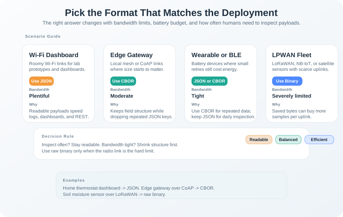
Read the scenario map as a fit test, not as a ladder of sophistication. If JSON fits with margin and operators need readable logs, stop there. Move to CBOR when the link is constrained but fields still vary, to Protocol Buffers when stable typed contracts matter more than ad hoc inspection, and to custom binary only when the byte budget leaves no practical alternative.
Worked Example: A 51-Byte LoRaWAN Payload
A vineyard deploys soil nodes. Each node reports a device ID and four readings: soil moisture, soil temperature, air temperature, and battery voltage. LoRaWAN at the slowest data rate (SF12, about 250 bits/s) allows roughly a 51-byte payload. The question is which format fits.
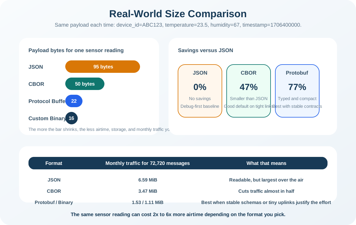
Per transmission at roughly 44 mA radio current, the CBOR message uses about 44 mA x 1.5 s = 66 mA-s (about 18 uAh), while the 8-byte binary message uses about 11 mA-s (about 3 uAh). The binary version cuts radio energy per message by roughly five to six times. Treat these as first-order estimates: real LoRaWAN airtime also includes preamble and symbol overhead, and total device lifetime is usually limited by sleep current and battery self-discharge, not radio time alone.
Try It: Size Your Own Message
Take a sensor you know. Write the message as JSON and count the bytes, then rewrite the same fields with short keys, then as integer-scaled values. Record where it would first fail a 51-byte LoRaWAN payload, and which step recovered the most space.
Incremental Practice
Beginner
For a Wi-Fi sensor that posts every minute, justify staying on JSON instead of switching to binary.
Intermediate
For a LoRaWAN node, convert a JSON message to short keys and integer scaling, and record the byte count at each step.
Advanced
Design a hand-packed layout for a 12-byte Sigfox uplink, including a version byte and reserved bits for one future field.
Payload Sizing Knowledge Check
A format that fits today still needs a versioned contract so future fields and older receivers can coexist.
10.5 Under the Hood: Encoding Mechanics, Schema, and Cost
The mechanics explain why the formats differ in size and why some changes are safe while others break deployed devices. Each format makes a different trade between readability, self-description, and bytes.
Airtime and Energy
Payload size becomes battery cost through two simple relationships on a constrained link:
airtime = payload_bytes x 8 / data_rate
energy_per_message ~= radio_current x airtime
These first-order estimates explain why halving a payload roughly halves transmission energy. They omit fixed overhead such as preamble, headers, and acknowledgements, so a very small payload saves proportionally less than the raw byte count suggests.
How the Formats Encode
CBOR is an IETF standard (RFC 8949, originally RFC 7049) and pairs naturally with CoAP on constrained networks. Protocol Buffers are a schema-compiled format common in gRPC services where the contract is stable and versioned. MessagePack is a similar binary-JSON bridge that needs no schema. XML remains in some legacy industrial and enterprise systems but is too verbose for tight radio links.
Integer Scaling Beats Floats
A common waste is sending every number as a 64-bit float. A temperature stored as 23.5 in IEEE 754 double precision takes 8 bytes. Stored as temperature x 10 = 235 in a 16-bit integer, it takes 2 bytes with identical precision for typical IoT ranges. Across a ten-field message that difference dominates the payload.
Schema Evolution
IoT fleets are rarely updated all at once. Devices, gateways, and cloud consumers may run different versions for a long time, so the format has to survive staged change.
- Add fields, do not repurpose them. New consumers use new fields; old consumers ignore what they do not understand. Never silently reuse a field for a new meaning.
- Keep meaning stable. A field name or number should keep the same unit and interpretation across versions.
- Version the contract. When a format cannot be self-describing enough, carry a layout or decoder version so the receiver knows how to read it.
- Test old and new. Run old producer to new consumer, new producer to old consumer, and any gateway conversion before deployment.
Common Pitfalls
-
Encoding numbers as strings. Sending
“23.5”instead of23.5forces string parsing, breaks numeric queries, and adds bytes. - Using floats for every field. Eight bytes per value is rarely needed; integer scaling keeps the precision and cuts the size.
- Choosing binary too early. Custom binary adds encoder, decoder, and debugging cost; pay it only when the link budget actually requires it.
- Ignoring schema evolution. Adding or renaming a field without a versioning rule can break consumers that have not been updated yet.
Custom Binary Knowledge Check
Format-to-Protocol Fit
A mature format choice is a chain of costs: link budget, readability, self-description, schema stability, and forward compatibility. A trustworthy payload records each one instead of treating the bytes as self-explanatory.
10.6 Summary
- A data format choice is a trade-off between human readability and byte efficiency; there is no single best format.
- Size the link first: maximum payload, data rate, and message cost decide how compact the format must be.
- Use the most readable format the link can afford, stepping from JSON to CBOR to custom binary only as the budget forces.
- On a constrained link, payload size drives radio airtime and transmission energy, so smaller messages save battery.
- Integer scaling and short keys recover most of the space that naive JSON and 64-bit floats waste.
- Schema evolution must be planned: add fields additively, keep meaning stable, version the contract, and test mixed versions.
The right IoT data format is the most readable one that still fits the link, with a documented decode contract so the receiver can reconstruct the meaning long after the bytes were sent.
10.7 See Also
Binary Data Formats
Go deeper on CBOR, Protocol Buffers, and custom binary encoding details and trade-offs.
Bitwise Operations and Endianness
Learn the byte-order, masking, and packing skills that custom binary layouts depend on.
Packet Anatomy
See how a formatted payload sits inside protocol headers, framing, and trailers.