38 WSN Papers Guide
Foundational Surveys, Energy Constraints, and Practical WSN Reading Lanes
38.1 In 60 Seconds
This chapter helps you read two foundational Wireless Sensor Network surveys without turning them into outdated hardware advice. Akyildiz et al. define the early WSN problem space: constrained nodes, radio-dominated energy use, multi-hop routing, and data-centric design. Yick et al. show how the field matured through platforms, operating systems, routing families, aggregation, sensing-area models, and deployment lessons.
38.2 Start With the Story
Start with a design review where a paper is useful only if the team can extract the claim, evidence, assumptions, and limits without turning it into folklore. The core idea in WSN Papers Guide is simple: paper reading for IoT is a disciplined way to connect research claims to architecture, WSN, protocol, and security decisions. This page focuses that idea on Guided reading of Akyildiz et al. and Yick et al. for understanding wireless sensor network foundations, node architecture. In everyday IoT, old networking and security papers still shape constrained stacks, cloud architectures, privacy models, and field validation expectations. Start simple: read for the problem, the method, the evidence, and the limits before importing a paper claim into a design.
38.3 Learning Objectives
By the end of this chapter, you will be able to:
- Read WSN surveys as historical design evidence rather than as current bill-of-material guidance.
- Explain why node energy, local processing, communication, and topology were central WSN concerns.
- Separate abstract WSN models from later hardware, operating-system, and protocol evidence.
- Compare Akyildiz’s field-setting view with Yick’s practical-maturity view.
- Build a reading record that preserves paper claims, assumptions, and follow-up checks.
- Connect WSN concepts to later IoT routing, low-power networking, edge processing, and device-lifecycle decisions.
38.4 Reading Contract
Use these papers to learn the design pressure behind low-power sensing systems. Do not copy old platform tables, protocol rankings, or energy ratios into a current project without target-hardware measurement and current protocol evidence.
38.5 Papers Covered
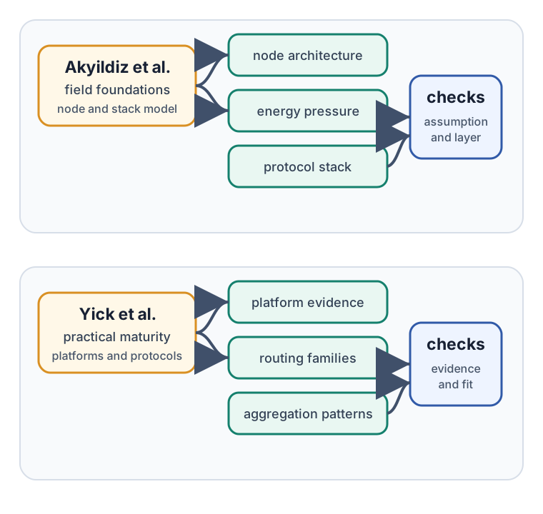
This guide focuses on two surveys because they let you read WSN history as an evolution from field definition to practical maturity.
I. F. Akyildiz, W. Su, Y. Sankarasubramaniam, and E. Cayirci, “Wireless sensor networks: a survey.”
- Venue: Computer Networks, 38(4), 393-422
- DOI: https://doi.org/10.1016/S1389-1286(01)00302-4
- Read for: WSN field definition, sensor-node architecture, protocol-stack pressure, energy-aware routing, and data-centric networking.
J. Yick, B. Mukherjee, and D. Ghosal, “Wireless sensor network survey.”
- Venue: Computer Networks, 52(12), 2292-2330
- DOI: https://doi.org/10.1016/j.comnet.2008.04.002
- Read for: practical platform comparison, operating-system and middleware context, routing families, aggregation patterns, sensing-area models, and open issues as the field matured.
38.6 Standards And Follow-Up Trail
These surveys are not standards. Use them to identify questions that later work had to answer:
- IEEE 802.15.4 for low-power wireless PHY/MAC context.
- RFC 4944 and RFC 6282 for IPv6 adaptation and header compression over low-power links.
- RFC 6550 for RPL routing in low-power and lossy networks.
- RFC 8180 and RFC 9030 for 6TiSCH minimal operation and architecture.
- WSN deployment papers such as habitat-monitoring studies for field evidence and failure modes.
The useful move is to ask: “What design pressure did the survey identify, and what later evidence would prove the design today?”
38.7 Lane 1: Akyildiz et al.
38.7.1 Why Read It
Akyildiz et al. are useful because they make the WSN problem space visible. The paper frames WSNs as systems where many small devices must sense, process, communicate, and survive under strong resource limits.
Read it to answer four questions:
- What is the assumed sensor-node architecture?
- Which design constraints come from energy, radio behavior, node count, and unattended operation?
- Why do data aggregation, clustering, and multi-hop paths appear so early in WSN research?
- Which parts of the protocol stack are changed by WSN constraints?
38.7.2 What To Extract
Node model: Record sensing unit, processing unit, transceiver, power unit, and any extra assumptions.
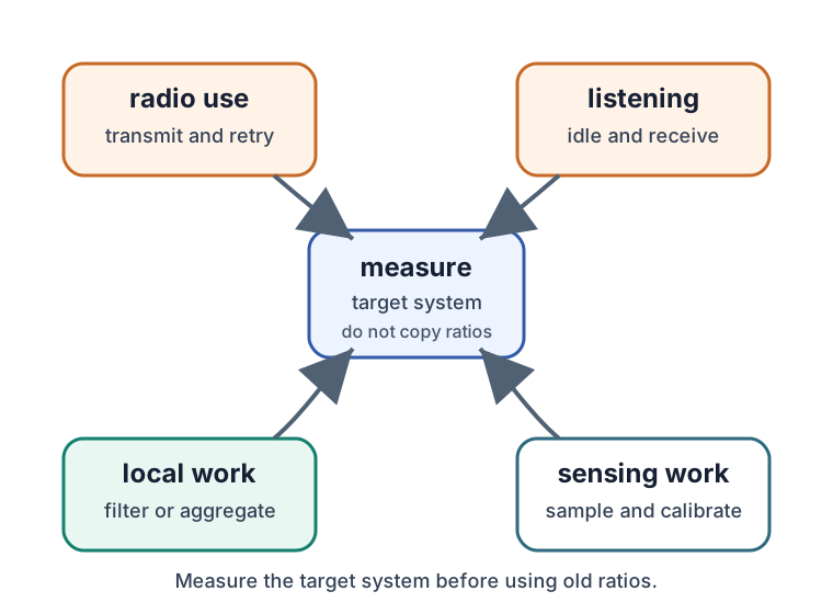
Dominant work: Record whether sensing, listening, local processing, or transmission is the limiting activity.
Network model: Record flat, hierarchical, cluster-based, data-centric, geographic, or multi-hop assumptions.
Evidence gap: Record what the paper assumes that would now require measurement or a later standards check.
38.7.3 Reading Route
- Read the abstract and introduction to identify the field definition.
- Read the node-architecture section before the protocol sections.
- In each protocol-stack section, ask what WSN constraint changed the design.
- When energy ratios or qualitative claims appear, record the assumption instead of copying the number.
- Finish by writing which claims still matter and which require modern measurement.
38.7.4 Checks While Reading
- Do not treat the paper as a current hardware guide.
- Do not reduce the paper to “radio is expensive.” Record listening, retransmission, synchronization, aggregation, and idle behavior too.
- Do not assume every early routing idea became a product protocol.
- Do not copy application examples without checking whether the sensing, maintenance, and data-path assumptions still hold.
38.8 Lane 2: Yick et al.
38.8.1 Why Read It
Yick et al. are useful because they show how WSN research became more practical after the early field-setting work. The paper compares platforms, operating systems, routing protocol families, aggregation approaches, sensing-area models, and research gaps.
Read it to answer four questions:
- Which WSN concepts became concrete platforms, protocols, or middleware patterns?
- Which routing families solve different constraints and which introduce new overhead?
- How do aggregation and local processing change what must be transmitted?
- Which open issues remained after early WSN practice matured?
38.8.2 What To Extract
Practical evidence: Record where the paper moves from concept to platform, implementation, or deployment lesson.
Protocol family: Record flat, hierarchical, location-based, data-centric, query-based, or quality-aware routing assumptions.
Aggregation pattern: Record where local processing reduces communication and where it may lose detail.
Sensing-area assumption: Record whether the paper assumes area, point, barrier, redundant, or sparse sensing.
38.8.3 Reading Route
- Read the introduction and compare the scope with Akyildiz.
- Skim platform and operating-system sections to see how abstract nodes became real systems.
- Read routing and aggregation sections as classification frameworks, not as rankings.
- Read sensing-area and connectivity material for assumptions about spatial evidence.
- Finish by mapping open issues to later IoT, low-power networking, security, and operations work.
38.8.4 Checks While Reading
- Do not treat platform comparisons as purchasing advice.
- Do not assume a routing protocol is useful because it has a large taxonomy entry.
- Do not ignore field operations: placement, maintenance, calibration, update, and data quality are part of the system.
- Do not import a mathematical model without stating the physical assumption it depends on.
38.9 Cross-Paper Synthesis
Read the two surveys together as a field-evolution story.
Akyildiz helps you see why WSN became a distinct research field. Yick helps you see which early ideas gained practical shape, which remained research-heavy, and which required later standards or deployment evidence.
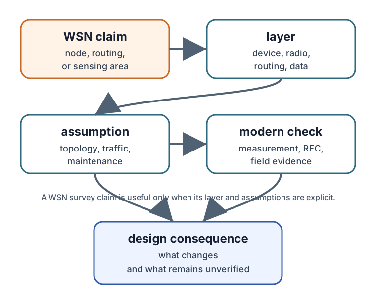
38.9.1 Synthesis Record
Use this format for each reusable claim:
- Paper: Akyildiz or Yick.
- Claim: The WSN design point in one sentence.
- Affected layer: Device, radio, MAC, routing, aggregation, application, sensing area, or operations.
- Assumption: Node capability, topology, traffic pattern, maintenance model, or spatial model.
- Modern check: Measurement, RFC, standards profile, deployment evidence, or operating process.
- Design consequence: What the claim changes in sensing schedule, packet volume, routing, local processing, update, or maintenance.
38.9.2 Example Synthesis
Claim: Local aggregation can reduce radio use when multiple nearby readings carry overlapping information.
Affected layer: Local processing, routing, and data quality.
Assumption: Nearby readings are similar enough that summary values preserve the decision signal.
Modern check: Measure target-device energy, compare raw versus aggregated data quality, and define what detail must remain available for troubleshooting.
Design consequence: Aggregation is useful only when the quality contract is explicit and the system keeps enough evidence for diagnosis.
38.10 Common Pitfalls
The surveys explain why communication often dominates WSN energy, but exact ratios depend on device, radio, payload, sleep state, channel, and software. Record the principle, then measure the target system.
Survey tables organize the literature. They do not prove that a routing family, aggregation method, or topology is the right design for your system.
Many early WSN papers focus on protocol behavior. Real systems also need placement records, calibration, updates, replacement plans, gateway recovery, and data-quality checks.
WSNs are not only networks. They exist to answer a sensing question. A routing design is not useful if it saves transmissions while losing the evidence the application needed.
38.11 Check Your Understanding
38.11.1 Knowledge Check: Akyildiz Reading Lens
38.11.2 Knowledge Check: Yick Reading Lens
38.11.3 Matching Check
38.11.4 Ordering Check
38.12 Deep Dive: Translate WSN Surveys Into Measurement Plans
A wireless sensor network is a collection of many small, battery-powered nodes that sense their surroundings and relay readings, often over multiple hops, to a sink or base station. WSNs are the research ancestor of much of IoT, and their papers return to one theme: energy is the scarce resource, so the whole network is engineered to conserve transmit, receive, idle-listen, sense, and compute time.
The most reusable WSN idea is not a specific protocol table. It is the discipline of writing down the system assumption behind a claim. Was the traffic periodic or event-driven? Were nodes fixed or mobile? Was the sink single, mobile, or replicated? Was packet loss modeled, measured, or ignored? Did the result depend on homogeneous nodes, synchronized sleep slots, or easy physical access for battery replacement? Those assumptions decide whether a survey claim transfers to a later IoT design.
| Claim type | Reading question | Evidence before reuse |
|---|---|---|
| Energy ratio | Which state dominates: transmit, receive, idle listening, sensing, or local processing? | Target-device current measurement in each state |
| Routing gain | Which topology, sink placement, traffic pattern, and failure model were assumed? | Delivery ratio, retransmissions, parent churn, repair time |
| Aggregation gain | What information is summarized, discarded, or delayed? | Data-quality comparison between raw and aggregated records |
| Sensing-area model | What physical coverage, redundancy, or calibration assumption is made? | Placement record, coverage test, calibration evidence |
| Deployment lesson | Which maintenance task is hidden by the paper model? | Battery replacement, firmware update, gateway recovery plan |
38.12.1 Energy-Saving Mechanisms
Because the radio is a major energy cost, WSN techniques mostly aim to turn it off, transmit less, or avoid wasteful receive time.
| Technique | What it does | Evidence to capture |
|---|---|---|
| Duty-cycled MAC | Radio sleeps, waking briefly to check for traffic | Sleep current, wake latency, missed event rate, synchronization overhead |
| Multi-hop routing | Short hops via neighbors to the sink | Delivery ratio, retry count, relay burden, repair behavior |
| Data aggregation | Combines readings in-network, such as average, maximum, count, or threshold state | Transmission reduction, error from summarization, diagnostic detail retained |
| Event-driven reporting | Sends only on change, threshold, or alarm state | False negatives, burst behavior, timestamp quality, recovery after missed events |
In-network aggregation shows the core WSN trade. Fifty temperature nodes in a field can each forward one reading toward the sink, creating a traffic concentration near the sink. If intermediate nodes compute an average, maximum, or count and forward one aggregated value, the network spends a little local computation to avoid a lot of radio time. That is useful only when the quality contract says the summary preserves the decision signal; a maintenance workflow may still need raw samples for fault diagnosis.
Survey tables should therefore be treated as triage maps. A flat routing family may be simple, a hierarchical or clustered family may reduce long-range traffic, and a geographic family may fit location-aware deployments, but none is “best” without topology, traffic, link-quality, maintenance, and data-quality evidence. If a claim depends on low-power links, check the relevant IEEE 802.15.4 profile and radio behavior. If it depends on IP over constrained links, follow 6LoWPAN and RPL material such as RFC 4944, RFC 6282, and RFC 6550. If it depends on time-slotted industrial operation, look at 6TiSCH work rather than assuming a generic WSN MAC.
38.12.2 Idle Listening And Energy Holes
Two under-the-hood facts drive WSN research. First, a major hidden energy cost is often idle listening, which keeps the radio on waiting for a packet that may never come. A radio in receive mode can draw current close to its transmit state, so a node that listens continuously drains quickly even if it rarely sends. Duty-cycled MAC protocols exist to eliminate idle listening by scheduling brief, coordinated wake-ups.
Second, multi-hop relaying creates the energy-hole or hotspot problem. Nodes closest to the sink must forward other nodes’ traffic, so they can deplete first; when they die, the sink can be cut off even though distant nodes still have power. In a linear pipeline reporting to a sink at one end, the node nearest the sink may relay all upstream traffic and exhaust its battery much earlier than the rest. A designer may add redundant nodes near the sink, rotate relay roles, change sink placement, or rebalance routing so useful lifetime is not bounded by one overloaded relay.
The under-the-hood reading question is whether the paper’s model closes the loop between physics, protocol state, and operations. A radio model that ignores receive current hides idle-listening cost. A routing model that averages energy across all nodes can hide sink-near depletion. A sensing-area model that assumes perfect coverage can hide calibration drift, failed nodes, vegetation, enclosures, and gateway outages. Those omissions are not always flaws in the paper; they are assumptions that must be carried into the review record.
Layer boundaries matter too. A MAC schedule can save energy but increase latency. A routing repair can restore connectivity but cause bursts of control traffic. In-network aggregation can lower packet volume but erase the raw evidence needed for anomaly diagnosis. A sink move can balance relay load but change custody of data and gateway availability. When the WSN literature reports an improvement, ask which adjacent layer paid for it.
For a modern IoT transfer decision, require five pieces of evidence: measured target-device current in sleep, receive, transmit, sensing, and local processing states; link-quality and retry data in the target environment; routing or parent-change behavior under failures; data-quality loss from filtering or aggregation; and an operations plan for placement, calibration, firmware updates, and battery replacement. That turns an old survey insight into a current engineering constraint.
38.13 Summary
Akyildiz et al. and Yick et al. are most useful when they explain why low-power sensing systems are designed around resource limits, communication behavior, local aggregation, routing assumptions, sensing-area evidence, and deployment maintenance. Read Akyildiz for field foundations. Read Yick for practical maturation. Use both to build review records, not to copy old platform details.
38.14 See Also
38.15 What’s Next
Next, continue through the remaining paper-reading guides and keep the same record format: paper claim, affected layer, assumption, modern check, design consequence, and unresolved verification step.
38.16 Key Takeaway
WSN papers should be read through node constraints, topology, energy model, routing behavior, deployment assumptions, and evaluation metrics. Energy and link realism decide whether results transfer.