19 Battery-Life Target Contracts
Turning Battery-Life Targets into Measured IoT Design Decisions
19.1 Start With a Battery-Life Contract
A battery-life target is a contract between the service promise, the source, the load, and the environment. If any part is vague, the final lifetime claim will be vague too.
Start by writing the contract as numbers: operating interval, peak pulse, average current, derating, brownout threshold, maintenance window, and the evidence needed before deployment.

Phoebe’s Why
This chapter’s own average-current budget – \(I_{avg,max}=C_{usable}/T\) – and its later coin-cell sections both work entirely in mAh and amps, and that is deliberate: mAh is a charge unit, a count of electrons moved, and the average-current math only needs charge. But two things this chapter lists as separate bullets, self-discharge and “mAh is not a complete battery specification,” are really the same underlying fact from a different angle: the cell’s energy in watt-hours is charge times the voltage it was delivered at, and that voltage is not constant over the discharge. Self-discharge quietly spends some of that charge before the load ever sees it, through the same chemistry, with no circuit current to log.
The Derivation
Instantaneous power and the energy actually delivered:
\[P(t) = V(t)\,I(t) \qquad E = \int P\,dt = \int V(t)\,I(t)\,dt\]
For the roughly constant currents this chapter’s ledgers already use, charge and energy separate cleanly:
\[Q = \int I\,dt \qquad E = Q\,\bar{V}, \qquad \bar{V}=\frac{1}{T}\int V(t)\,dt\]
So watt-hours equal the mAh rating only when multiplied by the average discharge voltage, not the fresh open-circuit voltage. Self-discharge shrinks the same \(Q\) before the load draws it, and a simple constant-rate model tracks it as:
\[Q(t) = Q_0\,(1-r)^{t}\]
where \(r\) is the fractional self-discharge rate per year.
Worked Numbers: This Chapter’s Own CR2032, Charge Versus Energy
- This chapter’s own 225 mAh CR2032 at its own nominal 3.0 V gives an energy ceiling \(E=0.225\times3.0=0.675\) Wh; at the 2.0 V brownout-region floor this chapter already uses, the lower bound is \(E=0.225\times2.0=0.450\) Wh. The true delivered energy sits between these bounds, closer to the upper one, because lithium-manganese dioxide cells like the CR2032 hold a comparatively flat discharge voltage for most of their life.
- Self-discharge, catalog-typical for this chemistry at about 1%/year, compounded over this chapter’s own ten-year target: \(Q(10)/Q_0=(0.99)^{10}=0.904\), a \(9.56\%\) loss of the rated 225 mAh – about 21.5 mAh – before any circuit ever draws a milliamp.
- Expressed the same way this chapter expresses its circuit currents, that loss is equivalent to a hidden average drain of \(21.5\ \mathrm{mAh}/(10\times8760\ \mathrm{h})=0.246\ \mu\mathrm{A}\) – next to this chapter’s own \(2.6\ \mu\mathrm{A}\) ten-year average-current allowance for the same cell, self-discharge alone consumes about \(9.5\%\) of that entire budget, invisibly, before the pulse-sag and reservoir-capacitor checks in this chapter even begin.
19.2 Energy-Aware Design Considerations
Energy design is not a calculator at the end of an IoT project. It is a design constraint that shapes the hardware, firmware, network behavior, enclosure, maintenance plan, and field test plan from the first architecture review.
The central question is simple: can the device deliver the required service for the required lifetime under realistic field conditions? The answer requires more than a battery capacity number. It requires a state-by-state current ledger, derated source assumptions, protocol behavior under poor coverage, and measurement evidence from the whole device.
19.3 Learning Objectives
By the end of this chapter, you will be able to:
- Convert a battery-life target into a maximum average-current budget.
- Build a current ledger for sleep, sensing, compute, radio, and exception states.
- Explain why source derating, peak current, and end-of-life voltage matter.
- Choose design changes based on the dominant energy drain rather than intuition.
- Evaluate protocol and duty-cycle choices against payload, interval, retry, and latency requirements.
- Specify measurement evidence needed before accepting a battery-life estimate.
- Review an IoT energy design for field risks without relying on generic claims.
- Battery capacity sets the energy budget; service requirements decide how quickly that budget may be spent.
- Average current is useful only when it includes every state that happens in the field.
- Sleep current often dominates long deployments because it runs almost all the time.
- Radio energy can dominate when messages are frequent, long, or retried.
- A larger battery hides design mistakes but does not fix leakage, retries, warm-up time, or poor measurement.
- A credible design has measured whole-device current and margin for temperature, aging, and worst-case behavior.
19.4 The Energy Design Gate
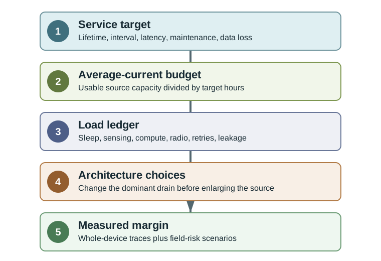
Use the same five gates for every battery-powered IoT device.
19.4.1 1. Service Target
Define the useful service before sizing the battery: sample interval, reporting interval, latency, local storage, maintenance window, and acceptable loss of readings.
19.4.2 2. Source Budget
Estimate usable capacity after derating. Include regulator efficiency, end-of-life voltage, temperature range, pulse-current limits, and shelf life.
19.4.3 3. Load Ledger
List every state that consumes current. The ledger must include sleep, sensor warm-up, compute, radio attach, retries, indicators, pull-ups, and debug hardware.
19.4.4 4. Design Levers
Change the dominant drain first. Shorten awake time, reduce leakage, batch messages, change protocol behavior, power-gate peripherals, or revise the service requirement.
19.4.5 5. Evidence Margin
Measure the whole device and compare it with the budget. Keep margin for battery aging, cold starts, field retries, firmware updates, and manufacturing variation.
19.5 From Lifetime Target to Current Budget
Start with the target lifetime and work backward.
For a battery with usable capacity \(C_{usable}\) in mAh and target life \(T\) in hours:
\[I_{avg,max} = \frac{C_{usable}}{T}\]
If a device must run for five years from a 2400 mAh source, and the design team reserves 30% for derating and margin, the usable capacity is:
\[C_{usable} = 2400 \times 0.70 = 1680\text{ mAh}\]
Five years is approximately \(5 \times 365 \times 24 = 43{,}800\) hours, so:
\[I_{avg,max} = \frac{1680}{43800} = 0.038\text{ mA} = 38\text{ uA}\]
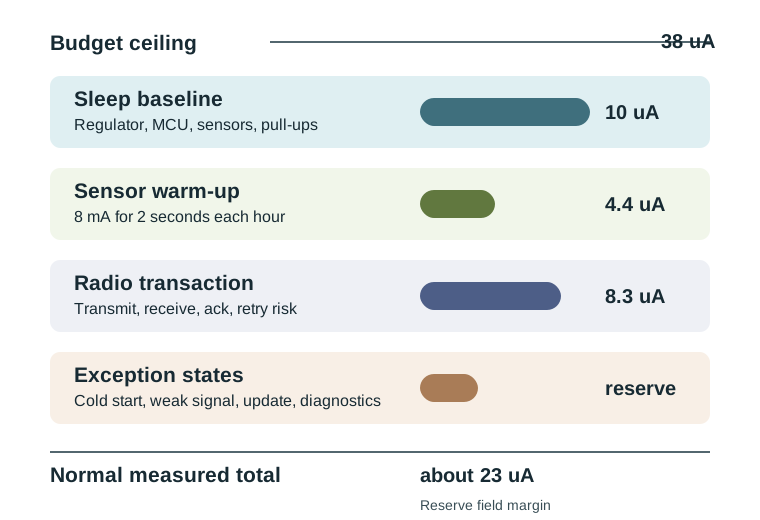
That 38 uA number becomes the design contract. It is not the sleep-current target alone; it is the maximum average current for the whole device across sleep, wake, sensing, compute, communication, and failure-recovery behavior.
19.6 Build the Load Ledger
A useful energy review separates states by current and time. The example below uses one hourly sensing and reporting cycle.
State
Current and Time
Average Contribution
Review Question
Sleep baseline
10 uA for nearly the full hour
About 10 uA average
Is this whole-board current, including regulator, sensor leakage, pull-ups, and disabled debug circuits?
Sensor warm-up
8 mA for 2 seconds each hour
About 4.4 uA average
Can the sensor be powered only when needed, or can warm-up time be shortened without reducing data quality?
Radio transaction
120 mA for 0.25 seconds each hour
About 8.3 uA average
Does this include join, attach, acknowledgement, retry, and poor-coverage behavior?
Normal total
Sleep plus sensing plus radio
About 23 uA average
Does the total stay below the 38 uA design contract with enough field margin?
The ledger shows why both sleep and active states matter. Sleep is the largest single state in this example, but the two short active states still use more than half of the available margin. If radio retries double the transaction time, or if sensor warm-up grows from 2 seconds to 8 seconds, the design can fail without any change to the battery.
19.7 Choose the Right Design Lever
Do not optimize the easiest number. Optimize the dominant drain.
If sleep dominates Measure whole-board sleep current, disable unused peripherals, check pull-up values, power-gate sensors, choose lower quiescent-current regulators, and remove debug leakage paths.
If sensing dominates Reduce warm-up time, lower sample frequency, cache calibration, use event-driven sampling, or choose a sensor that meets accuracy needs with less standby and warm-up current.
If radio dominates Batch payloads, reduce retransmissions, tune acknowledgement behavior, improve antenna placement, choose a protocol that matches payload size and range, or process locally before sending.
If exceptions dominate Measure reconnect storms, firmware update windows, failed joins, low-temperature starts, and diagnostic modes. Rare events can control field battery life if they last minutes.
19.8 Source Selection Is More Than Capacity
A battery with a large mAh rating can still be the wrong source. Review these constraints before accepting a source choice:
- Usable capacity: Derate for temperature, aging, discharge rate, regulator efficiency, and end-of-life voltage.
- Peak current: Radio bursts can pull voltage below the device minimum even when average current looks safe.
- Self-discharge: Multi-year devices need a source whose storage loss is small compared with the load budget.
- Temperature range: Cold conditions reduce usable capacity and increase internal resistance.
- Recharge or replacement model: A rechargeable product has a different design contract than a sealed field node.
- Mechanical and service limits: Size, connector reliability, hazardous locations, and field access can dominate the source decision.
The mAh rating is measured under defined conditions. It does not prove that the battery can supply radio bursts, survive the deployment temperature range, or keep voltage above the device minimum at end of life. Always translate source data into usable capacity and peak-current evidence for the actual load.
19.9 Protocol and Workload Decisions
Communication energy depends on the workload, not only the protocol name. A protocol that is efficient for one-byte status messages may be inefficient for firmware updates, and a protocol with low transmit current may still waste energy if it retries often in the deployment environment.
Use these questions before choosing the radio behavior:
- Payload size: Is the message a small state update, a time series batch, a feature vector, or raw sensor data?
- Interval: Does the device report every few seconds, every hour, or only on events?
- Reliability: Are acknowledgements, confirmed delivery, or local buffering required?
- Coverage: What happens at the edge of range, inside enclosures, or during interference?
- Latency: Can the device wait for an efficient send window, or must it wake on demand?
- Local processing: Can the device send events or features instead of raw data?
The common “send less, sleep more” rule is useful, but it is incomplete. A design that sends less often may need longer sensor warm-up, larger local storage, or stronger reliability logic. Review the whole ledger.
19.10 Measurement Loop
Energy estimates become credible only after measurement. A spreadsheet can guide design, but a power trace catches firmware states, board leakage, retry behavior, and timing that the spreadsheet missed.
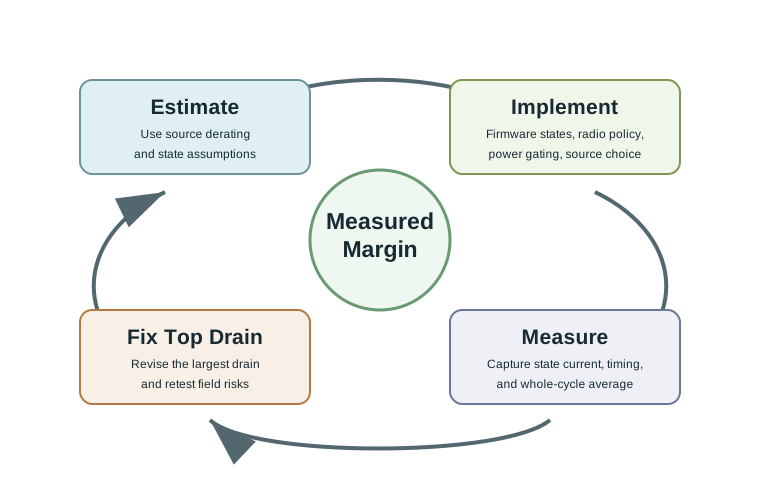
Measure at three levels:
- State current: Sleep, sensor warm-up, compute, radio transmit, receive, retry, firmware update, and diagnostic mode.
- State timing: How long each state lasts in normal and poor-condition cycles.
- Whole-cycle average: A complete cycle trace that includes all transitions and recovery paths.
Record the current trace, cycle script, firmware version, supply voltage, temperature condition, radio configuration, payload size, and retry policy. Without those details, another engineer cannot reproduce or challenge the battery-life estimate.
19.11 Try It: Estimate the Duty-Cycle Contract
Use the estimator before accepting a lifetime number from a spreadsheet. Change the wake interval, sleep current, active-state durations, usable capacity, temperature derating, and self-discharge, then compare the estimated life with the target average-current budget. The useful result is not just the years shown at the top; it is the dominant state and the margin that would have to be proven by measurement.
19.12 Worked Example: Environmental Node Review
Requirement: Outdoor environmental node, one sample and one report per hour, five-year service target.
Energy contract: 2400 mAh source, 30% reserved for derating and field margin.
\[I_{avg,max} = \frac{2400 \times 0.70}{5 \times 365 \times 24} \approx 38\text{ uA}\]
Measured normal cycle:
- Sleep baseline: 10 uA for almost the full hour.
- Sensor warm-up: 8 mA for 2 seconds.
- Radio transaction: 120 mA for 0.25 seconds.
Average contribution:
- Sleep: about 10 uA.
- Sensor warm-up: 8 mA for 2 seconds per hour gives about 4.4 uA average.
- Radio: 120 mA for 0.25 seconds per hour gives about 8.3 uA average.
- Total: about 23 uA.
Review result: The normal cycle fits the 38 uA contract. The review is not finished until the team measures cold start, weak-signal retries, firmware update mode, and whole-board sleep after sensors and debug circuits are disabled.
19.13 Energy Design Review Checklist
Use this checklist before approving a battery-powered IoT design.
Requirement The service target states lifetime, reporting interval, latency, storage behavior, maintenance model, and acceptable data loss.
Budget The source capacity is derated, and the maximum average-current budget is written as a number in uA or mA.
Ledger The current ledger includes sleep, active work, radio behavior, exceptions, indicators, pull-ups, regulators, and disabled-but-powered peripherals.
Dominant Drain The proposed optimization targets the largest measured contributor, not the most visible component.
Peak Load Radio bursts and startup current do not pull the supply below the device minimum voltage at end of life.
Measurement Whole-device traces confirm state current, state timing, average current, and field-risk scenarios.
19.14 Common Pitfalls
A firmware loop may run for only seconds per day, while regulator quiescent current, pull-ups, sensor leakage, and debug circuits run all day. Measure whole-board sleep current before celebrating active-mode savings.
Typical values rarely include temperature extremes, poor coverage, aging, manufacturing spread, or board-level leakage. Use typical values for early estimates, then replace them with measured and derated values.
Average current can look safe while a radio burst resets the device because the battery voltage sags. Check pulse-current capability and the minimum voltage of the full system.
Reconnect storms, failed joins, long sensor warm-up, firmware updates, and user diagnostics can drain more energy than the normal cycle. Include those states in the ledger or justify why they are excluded.
19.15 Knowledge Check
19.16 Quiz: Finding the Failing Energy Assumption
19.17 Matching Quiz: Design Consideration to Energy Impact
19.18 Ordering Quiz: Energy-Aware Design Review
19.19 Label the Diagram: Energy Design Evidence
19.21 What’s Next
Choose batteries and power sources using capacity, pulse current, derating, and service constraints.
Energy Cost of Common Operations
Compare compute, storage, sensing, and communication costs in IoT workloads.
Read measured case patterns and learn how energy lessons transfer between deployments.
19.22 A Coin Cell’s Real Limit Is Its Resistance, Not Its mAh
A CR2032 coin cell is labeled around 220 mAh, and it is tempting to treat that as a fuel tank you can drain any way you like. But that number is measured at a very low continuous drain - a fraction of a milliamp - down to a 2.0 V cutoff. A radio that pulses several milliamps for a few milliseconds is a completely different load, and the cell's internal resistance, not its stored charge, is what usually ends the design.
Every cell has an internal resistance. In a CR2032 it starts around 10-15 ohms when fresh and climbs to many tens of ohms as the cell depletes. Ohm's law then turns each current pulse into a voltage drop right at the terminals. When that drop pulls the rail below the processor or radio brownout threshold, the device resets - even though most of the labeled capacity is still inside the cell.
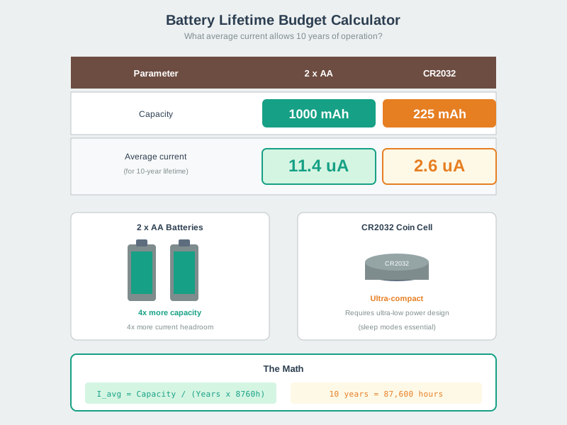
For example, the ten-year average-current allowance for a 225 mAh CR2032 is only about 225 / (10 x 8760) = 2.6 uA. A beacon may meet that average by sleeping almost all the time, yet still draw a 10 mA transmit pulse. At 40 ohms of aged internal resistance that pulse sags about 0.010 x 40 = 0.4 V, so a 2.7 V cell looks like 2.3 V during the burst. The lifetime budget and the pulse-sag budget therefore have to pass together.
Intuition only: a coin cell can hold plenty of charge and still be unable to deliver it fast enough. Always check the peak pulse against the cell's resistance, not just the average current against its capacity.
Two Different Questions
Enough energy?
Average current versus usable capacity sets how long the charge lasts. This is the mAh question.
Enough current?
Peak pulse times internal resistance sets the voltage sag. This is the ohms question the label hides.
Rising resistance
Internal resistance grows as the cell empties, so the sag gets worse exactly when the cell is already weaker.
The reservoir fix
A capacitor across the cell supplies the fast pulse so the cell only has to provide the slow average.
Overview Knowledge Check
19.23 Check The Pulse, Not Just The Average
Two checks decide a coin-cell radio design. The sag check uses Ohm's law: V_sag = I_pulse x R_internal. The reservoir check sizes a bulk capacitor to hold the pulse so the cell only supplies the average: C = I_pulse x t_pulse / dV_allowed.
Worked Example: BLE Beacon On A CR2032
The radio pulse is 10 mA for 5 ms per advertising event. The average current is low, so the mAh budget looks comfortable - but the pulse is the problem.
- Fresh cell, R = 10 ohm:
V_sag = 0.010 x 10 = 0.1 V. From a 3.0 V terminal that is 2.9 V under pulse - fine. - Aged cell, R = 40 ohm:
V_sag = 0.010 x 40 = 0.4 V. If the open-circuit voltage has fallen to 2.7 V, the rail dips to 2.3 V under pulse, approaching a typical 2.0-2.2 V brownout with capacity still inside. - Reservoir capacitor for 0.2 V droop:
C = 0.010 x 0.005 / 0.2 = 250 uF. This capacitor delivers the pulse; the cell then recharges it slowly at the average current, so the cell's high resistance no longer causes the sag.
With the reservoir capacitor in place, the design finally gets to use the cell's stored charge, because the cell is asked only for the average current it can comfortably supply.
The reservoir is not free, so review its leakage and effective series resistance too. A 250 uF capacitor that leaks 1 uA consumes 1 uA x 10 years x 8760 h/year = 87.6 mAh, almost 40% of a 225 mAh CR2032 before the load does any useful work. The right fix is a low-leakage reservoir sized for the pulse width, not simply the largest capacitor that fits on the board.
Coin-Cell Pulse Ledger
Practitioner Knowledge Check
19.24 Usable Capacity Depends On Your Brownout Threshold
For a pulsed load, "usable capacity" is not a fixed fraction of the label. It is set by the point where the sagging pulse voltage first touches your brownout threshold. Because internal resistance rises as the cell depletes, the sag grows over life: a pulse that dropped 0.1 V when fresh may drop 0.5 V or more near the end. The higher your pulse current and the higher your brownout voltage, the earlier that crossing happens - and the more of the rated 220 mAh you leave stranded in the cell.
This is why a design must pass two independent checks. The average-current check tells you whether there is enough energy for the target lifetime. The peak-pulse check tells you whether the cell can deliver each burst without browning out. A design can pass the first and fail the second: comfortable average current, plenty of mAh, and still an early death because the aged cell can no longer swallow the transmit pulse. A reservoir capacitor, a lower-resistance cell chemistry, or a gentler radio setting moves the crossing later and unlocks more of the stored charge.
A quick threshold calculation shows the effect. If the open-circuit cell is at 2.6 V and the radio pulse is 10 mA, a 2.4 V brownout allows only (2.6 - 2.4) / 0.010 = 20 ohm before reset. A 2.0 V brownout allows (2.6 - 2.0) / 0.010 = 60 ohm. The same cell and the same average current can therefore deliver very different field life depending on the minimum voltage of the regulator, microcontroller, sensor, and radio chain. Treat the brownout threshold as a design variable to review, not as a hidden firmware detail.
What Actually Sets Usable Capacity
Brownout threshold
A higher minimum operating voltage is reached sooner under sag, stranding more charge.
Pulse magnitude
Bigger transmit pulses sag more for the same resistance, cutting usable capacity.
Resistance growth
Internal resistance climbs with depth of discharge, so the sag is worst near the end of life.
Two-check rule
Pass the average-current energy check and the peak-pulse voltage check. Passing only one is not enough.
Under-the-Hood Knowledge Check
19.25 Summary
This chapter collects the main considerations for energy-aware IoT design: energy budgets, power sources, duty cycles, communication costs, environmental limits, maintenance, and measurement evidence.
19.26 Key Takeaway
Treat energy as a first-class requirement. Define lifetime, service level, power source, maintenance model, and measurement plan before choosing hardware or writing firmware.