6 Low-Power Design Strategies
Sleep Policy, Duty Cycling, Power Gating, and Firmware Discipline
6.1 Start With the Sleeping Device
The cheapest energy is the energy a device never draws. A low-power design begins by asking what must stay awake, what may sleep, and what event is allowed to wake the system again.
The simple route is service policy first, wake policy second, power states third, and measurement last. If a strategy cannot be seen in the trace, it is still only a claim.

Battery Bruno
“A strategy that isn’t in the trace is still just a claim — show me the charge it actually saved.”
Here Bruno follows the budget past sleep mode, into the radio and clock choices that decide whether the savings survive contact with real firmware.

Phoebe’s Why
Later in this chapter, a bus pull-up feeding a depowered sensor’s protection diode is sized with plain Ohm’s law: divide the rail voltage by the resistor and call it the leak. That is a fair first pass, but the current is not flowing into a dead short at 0 V – it is flowing into a forward-biased silicon junction, and a forward-biased junction holds its own terminal near a fairly constant voltage almost regardless of current, the way a spillway holds a fixed water level no matter how much flow passes over it. The pull-up resistor and that junction form a voltage divider of sorts: some of the 3.3 V rail is dropped across the resistor, and a roughly fixed slice is dropped across the diode. Leaving that slice out overstates the leak – not by a lot, but by exactly the diode’s own forward-voltage physics, which is worth knowing before trusting the number to three figures.
The Derivation
The naive estimate treats the far end of the pull-up as a 0 V short:
\[I_{naive} = \frac{V_{rail}}{R_{pullup}}\]
A forward-biased silicon junction instead holds a roughly constant drop \(V_f\) (a simplification of the diode’s exponential \(I\)-\(V\) law that is accurate enough for a leakage estimate), so the resistor only has to supply the remaining voltage:
\[I_{corrected} = \frac{V_{rail}-V_f}{R_{pullup}}\]
Worked Numbers: This Chapter’s Own 4.7 kΩ Pull-Up
- This chapter’s own naive figure: \(I_{naive}=3.3/4700=0.702\) mA – matches the “about 0.70 mA” already stated later in this chapter.
- Corrected for a catalog-typical silicon protection-diode drop, \(V_f\approx0.6\) V: \(I_{corrected}=(3.3-0.6)/4700=0.574\) mA – about \(18.2\%\) lower than the naive figure.
- Over the same two-line, 60 s sleep interval this chapter uses elsewhere: \(0.574\times2\times60=68.9\) mA-s corrected, versus \(0.702\times2\times60=84.3\) mA-s using the uncorrected per-line worst case – still two to three orders of magnitude above the 0.6 mA-s a 10 uA processor sleep would cost over the same interval.
- The honest bottom line: the diode-drop correction changes the leak estimate by less than a fifth, and it does not change this chapter’s conclusion at all – gate the whole island, rail and pull-ups and signals together. What it does change is whether the number quoted for that leak is defensible to one significant figure or to three.
6.2 Low-Power Design Strategies
Low-power design is not a single sleep-mode API call. It is a system policy that controls when the device wakes, what it powers, how long it stays active, and how quickly it returns to a measured low-current state.
This chapter focuses on the decisions that move an IoT node from a plausible budget to a working low-power design: sleep selection, duty-cycle policy, peripheral power gating, firmware timing, radio batching, and measurement discipline.
6.3 Learning Objectives
By the end of this chapter, you will be able to:
- Select a sleep mode from wake latency, state retention, and wake-source requirements.
- Design time-based, event-driven, and adaptive duty-cycle policies.
- Identify hidden loads from GPIOs, pull-ups, regulators, sensors, LEDs, and radios.
- Use power gating and state reinitialization without corrupting measurements or firmware behavior.
- Decide when batching, filtering, or local processing reduces radio energy.
- Explain when clock or voltage scaling helps and when it only stretches active time.
- Verify a low-power strategy with a whole-device current trace.
- The deepest sleep mode is not always best; wake latency, retained state, and wake-source support matter.
- Duty cycling reduces average current only if active work is short and sleep current is actually low.
- Peripherals can dominate sleep current unless they are disabled, held in a known state, or power-gated.
- Radio energy includes startup, association, receive windows, retries, and acknowledgments, not only transmit current.
- Every optimization claim should be checked against a before/after current trace.
Chapter path:
- First you choose a sleep state from wake source, wake latency, retained state, and whole-device current instead of from the lowest datasheet number alone.
- Then you turn the service requirement into a time-based, event-driven, hybrid, or adaptive duty-cycle policy and keep transition cost in the ledger.
- Next you control the loads that stay awake around the MCU: sensors, pull-ups, radios, indicators, rails, and reinitialization steps.
- Finally you verify the release with a trace that labels sleep, wake, sensing, radio, retries, and recovery states.
Checkpoints mark the review decisions; the worked policy review, Ada audit, and power budget calculator carry the detailed arithmetic.
At very low duty cycles, silicon leakage sets the floor. MOS transistors do not turn off as ideal switches: subthreshold current falls below the threshold voltage, but it does not become zero. Raising threshold voltage can reduce off current, but it also reduces available on current and can slow the active work that the node is trying to finish quickly.
Some chip families, including fully depleted silicon-on-insulator processes, expose forward or reverse body-bias modes to shift threshold voltage after fabrication. Treat that as chip-selection evidence rather than a magic firmware setting. Record the supported bias modes, retained state, sleep current, wake time, active-current penalty, and measured board leakage. If the board still leaves regulators, pull-ups, sensors, or debug circuits biased, body bias will not rescue the battery-life claim.
6.4 Strategy Stack
Low-power design works best when decisions are layered from service policy down to board leakage.
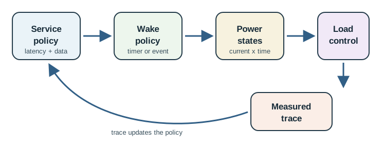
6.4.1 Service Policy
Define reporting interval, latency, data quality, and missed-event tolerance before choosing the sleep mode.
6.4.2 Wake Policy
Choose periodic wake, event wake, hybrid wake, or adaptive wake based on what the application must notice.
6.4.3 Power States
Map each firmware state to current, duration, retained memory, and wake source.
6.4.4 Load Control
Power-gate sensors, radios, indicators, and external circuits when they are not needed.
6.5 Sleep-Mode Selection
Sleep-mode selection is a requirements decision. A mode is viable only if it preserves the state you need, supports the wake source you need, and wakes quickly enough for the service requirement.
 Checkpoint: Sleep Policy Fit
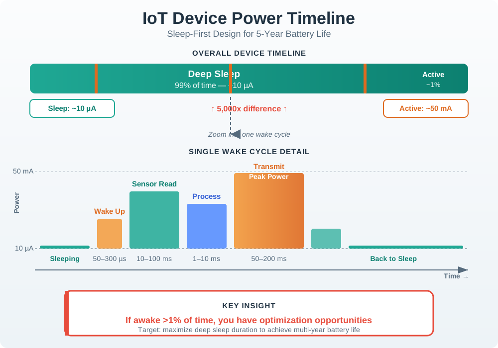
Before accepting a sleep mode, write down the allowed wake source, wake latency, retained state, full-cycle current trace, and the service interval it protects. The chapter’s 99% sleep example works only because deep sleep is paired with short active bursts and a measured low floor.
Mode Family
Use When
Watch For
Evidence To Capture
Idle or wait-for-interrupt
Wake must be nearly immediate and peripherals stay active.
Milliamps of standby current can destroy long-life budgets.
Idle current, interrupt latency, peripheral state list.
Light sleep
Frequent wake events need quick resume and retained RAM.
Retained clocks and peripherals may keep current high.
Sleep current, resume time, enabled clocks.
Deep sleep
Wake intervals are seconds to hours and limited state retention is acceptable.
Boot and reinitialization cost may dominate frequent wakes.
Full-cycle trace, wake cause, initialization time.
Shutdown or hibernate
Events are rare and only a small wake circuit must remain alive.
Full reboot, lost state, and limited wake pins.
Off current, wake reliability, state recovery test.
6.6 Duty-Cycle Policies
Duty cycling controls when the device spends energy. Start with the service requirement, then choose the simplest policy that meets it.
6.6.1 Time-Based
Wake on a fixed schedule. Use for slow-changing sensing where missing a short event is acceptable.
6.6.2 Event-Driven
Wake on an interrupt, comparator, sensor threshold, button, or radio event. Use when the event itself defines when work is needed.
6.6.3 Hybrid
Combine a watchdog timer with event wake. Use when the device must report health even if no event occurs.
6.6.4 Adaptive
Change the interval based on measured change rate, battery margin, harvested energy, link quality, or operational mode.
A temperature node reports every 10 minutes, but the environment changes slowly overnight.
Start with the required service: no more than 30 minutes between normal reports, and immediate reporting only when temperature crosses an alert threshold. A hybrid policy fits:
- Wake every 30 minutes for a health report.
- Let a low-power comparator wake the MCU if the threshold is crossed.
- Batch routine samples into one radio session.
- Record battery voltage and retry count with each report.
- Verify that the comparator and pull-up network do not exceed the sleep-current budget.
The policy saves energy because it removes unnecessary scheduled radio sessions while still preserving the alert requirement.
6.7 Folded Duty-Cycle Math Notes
Use duty-cycle math as a review ledger, not as a slogan. The basic average-current estimate is:
I_avg = (I_active * t_active + I_sleep * t_sleep) / (t_active + t_sleep)That estimate is only useful when the measurement record includes wake time, sensor stabilization, radio join time, retries, queue flushes, and the real sleep current of the whole board. Sleep current often dominates long-life designs: a small always-on regulator, pull-up, LED, sensor rail, or wake circuit can erase the benefit of a shorter active window.
Current-only math is a shortcut, not the definition of energy. It is defensible when all compared states use the same rail and regulator path; it is risky when battery voltage changes, a regulator burns the difference as heat, or the MCU is allowed to run across a wide supply range. In those cases, convert the state ledger to power or charge at the actual rail conditions before turning it into a battery-life claim.
Treat transition time as its own ledger term when the wake period is short. A BLE node that wakes once per second might sleep for about 999.6 ms at 4.8 uA, transmit and run the CPU for 0.3 ms at 14.6 mA, and spend another 0.14 ms moving the radio into transmit at 7 mA. The transition term is only about 1 uA-s, but it sits next to a sleep term of about 4.8 uA-s and an active term of about 4.4 uA-s. Leaving it out can make the cycle look roughly ten percent cheaper than the device actually measures.

Ada’s Ledger
Use the same one-second BLE cycle numbers from the paragraph above. Convert each duration to seconds, convert mA to uA where needed, then multiply current by time.
Formula
Charge (uA-s) = current (uA) x time (s).
I_avg = total charge / cycle time.
- Sleep: 999.6 ms = 0.9996 s, so 4.8 uA x 0.9996 s = 4.79808 uA-s.
- Active transmit and CPU: 14.6 mA = 14,600 uA and 0.3 ms = 0.0003 s, so 14,600 uA x 0.0003 s = 4.38 uA-s.
- Radio transition: 7 mA = 7,000 uA and 0.14 ms = 0.00014 s, so 7,000 uA x 0.00014 s = 0.98 uA-s.
- Total with transition: 4.79808 + 4.38 + 0.98 = 10.15808 uA-s; over 1 s, the average is 10.15808 uA, or about 10.16 uA.
- Total without transition: 4.79808 + 4.38 = 9.17808 uA-s; over 1 s, the average is 9.17808 uA, or about 9.18 uA.
- Difference: 10.15808 - 9.17808 = 0.98 uA, and 0.98 / 10.15808 = 0.0965, so omitting the transition hides about 9.7% of the measured average current.
The engineering lesson is not that every BLE product has this exact budget. It is that short transition states can be large enough to change the release decision, so the current trace should label them instead of folding them into a vague active bucket.
Checkpoint: Duty-Cycle Ledger
Review the duty cycle as charge per cycle, not as a slogan about sleeping more. In the BLE example, sleep contributes 4.79808 uA-s, active work contributes 4.38 uA-s, and the 0.98 uA-s transition term changes the average from about 9.18 uA to about 10.16 uA.
Use the wake policy to match the service contract:
| Policy | Use when | Review risk |
|---|---|---|
| Fixed interval | Slow sensing can tolerate bounded reporting delay. | Over-optimizing the interval while ignoring boot and radio overhead. |
| Event-driven | The event itself defines when work is needed. | Unbounded interrupts or a noisy threshold can drain the battery. |
| Hybrid | The system needs both immediate events and periodic health evidence. | Health reports, retry budgets, and event wakes compete for the same charge budget. |
Every low-power release should include field derating: battery chemistry, temperature, aging, link quality, and failure retries usually decide whether the lab duty cycle survives deployment.
6.8 Peripheral Power Gating
The MCU may be in deep sleep while sensors, pull-ups, level shifters, indicators, or a radio module continue drawing current. A low-power design needs a load inventory.
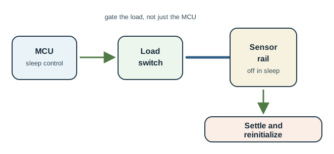
GPIO states are deliberate No floating inputs, accidental pull-ups, LEDs, or external loads should remain undefined during sleep.
Sensors are actually off Use enable pins or load switches when standby current exceeds the sleep budget.
Rails settle before reading After power-up, allow sensor warm-up and ADC/reference settling before trusting measurements.
State is rebuilt after wake Deep sleep may reset bus configuration, sensor registers, and radio state. Reinitialize before use.
6.9 Firmware Timing Discipline
Low-power firmware should make the active window short, deterministic, and measurable.
// Pseudocode pattern for a measured low-power cycle.
wake_cause = read_wake_cause();
start_trace_marker("wake");

enable_required_rails();
wait_for_sensor_settle();
sample = read_sensor();

if (should_report(sample, wake_cause)) {
    radio_on();
    send_batched_report(sample);
    radio_off();
}

disable_required_rails();
save_minimal_state();
schedule_next_wake();
enter_sleep();
Keep the active path boring. Avoid unbounded retries, blocking delays, unnecessary scans, debug output, and initialization work that could have been cached or skipped safely.
6.10 Radio and Data Strategy
The radio is often the highest-current state, but the fix is not always “use a different radio.” First reduce avoidable radio-on time.
6.10.1 Batch
Send several readings in one session when latency allows. This amortizes startup, association, and receive-window costs.
6.10.2 Filter
Transmit only changed, threshold-crossing, or summarized values when raw history is not required.
6.10.3 Bound Retries
Retry policies need a budget. Unlimited retries convert weak coverage into rapid battery depletion.
6.10.4 Separate Health From Data
Low-rate health reports can prove the node is alive without transmitting every raw sample.
Cellular batching is the same fixed-cost problem with a larger state machine. An LTE-style modem may move from idle into continuous reception, then through short and long DRX windows before it can return to the low floor. If the application can send two small records every 60 seconds instead of one small record every 30 seconds, the useful payload doubles while the expensive on, listen, tail, and release path is paid less often. Accept that trade only when the added data age is inside the service contract and the batch still preserves sequence numbers, alarm flags, and retry evidence.
Bruno’s Power Budget
- Draw: two records batched every 60 s carry the same total payload as one every 30 s, but pay the on/listen/tail path half as often.
- Sleep: every extra second the radio stays on is charge stolen straight from the sleep floor’s savings.
- Life: GSM-class links run on the order of 10,000 nJ/bit – worth checking before trusting cellular reach over a shorter local hop.
Short-range radios need the same state ledger. A sender pays transmit electronics and the RF power amplifier; a receiver pays receive electronics and often idle-listening time; the channel adds path loss and required SNR based on rate, BER target, and modulation. At long range, RF transmit energy may dominate. At very short range, receiver electronics, startup, acknowledgments, and listening windows can dominate instead.
Use technology tables as review prompts, not universal rankings:
| Radio comparison point | Representative review signal | What it should make you check |
|---|---|---|
| GSM-like long range | Around mile-scale range, hundreds of kbps, high transmit power, and order-of-10000 nJ/bit energy | Whether cellular reach is worth the radio-on time, attach cost, and service ownership. |
| Wi-Fi-like local links | High rate can make nJ/bit look good for large transfers, while receive, scan, join, and AP coordination still cost energy | Whether the workflow sends enough useful data per wake to justify the connection path. |
| 802.15.4 or Bluetooth-class links | Lower power and shorter range can fit sensor traffic, but receive windows, retries, and parent or gateway availability still matter | Whether the installed link, duty cycle, and command latency match the product requirement. |
For an embedded endpoint, “where the power goes” depends on the workload. One design may spend most calendar time asleep while a small transmit slice dominates charge; another may spend the budget in sensor warm-up or LEDs. Start with a back-of-the-envelope state budget, then validate it with real power measurements for sleep, sensing, transmit, receive, retry, and recovery states. The pie chart is not proof until the measured trace agrees with it.
6.11 Clock and Voltage Scaling
Dynamic voltage and frequency scaling can reduce instantaneous power, but it is not automatically an energy win. If lower frequency stretches the active window enough, the total energy may stay the same or increase.
Use clock or voltage scaling when:
- The workload has slack before the next deadline.
- The lower-power mode still finishes and returns to sleep early.
- Peripheral timing, radio deadlines, ADC accuracy, and bus clocks remain valid.
- The before/after trace shows lower charge per cycle, not just lower peak current.
Do not use it as a substitute for sleep, power gating, or radio batching.
Clock selection is also a firmware evidence item, not just a datasheet feature. A SAM4L-style Cortex-M design may expose run, sleep, wait, and retention modes, plus clock sources such as a 32 kHz oscillator, a 116 kHz system clock, a 1 MHz RC clock, and a 12 MHz fast RC clock. Use the slowest source or divider that still meets UART, SPI, ADC, radio, and interrupt timing requirements, then record the current and wake latency for that exact mode. Vendor-specific low-power states and clock trees are not portable across MCU families, so the review record should name the silicon, enabled clocks, retained peripherals, and measured charge per useful cycle. The same record should justify cost: a larger MCU or SoC may save active energy for one workload, but it still needs evidence that the added memory, buses, accelerators, or radio features are worth their price and sleep-floor consequences.
Bruno’s Power Budget
- Draw: a SAM4L-style part offers 32 kHz, 116 kHz, 1 MHz, and 12 MHz clock sources – pick the slowest one that still meets timing.
- Sleep: a faster clock only helps if it finishes sooner and returns to sleep earlier.
- Life: record current and wake latency for the exact mode used – vendor low-power states don’t port across MCU families.
6.12 Measurement Checklist
Measure the whole device Include regulators, sensors, radios, pull-ups, LEDs, debug probes, and board leakage.
Mark firmware states Use GPIO trace markers or logs so the current trace can be mapped to wake, sense, transmit, and sleep.
Check wake frequency Count actual wake events, retries, resets, and failed joins instead of assuming the ideal schedule.
Compare charge per cycle Judge optimization by total charge per reporting cycle, not by one impressive low-current state.
Checkpoint: Load And Firmware Control
A low-power claim is not ready until the board inventory and firmware path agree: unused rails are off, GPIOs are known, sensors settle before sampling, retries are bounded, and the trace shows that the code returns to sleep instead of waiting in a delay loop.
6.13 Common Pitfalls
Deep sleep can save standby current, but frequent wakes may spend significant energy on boot, clock setup, sensor warm-up, and radio rejoin. Measure the full cycle.
Sensors, level shifters, pull-ups, radios, LEDs, and regulators can draw more current than the sleeping MCU.
A delay keeps the processor or scheduler active. Replace idle waiting with an appropriate sleep state.
Lower peak current is not enough. The optimization must reduce the area under the current-versus-time trace.
Weak radio links, stuck interrupts, sensor faults, reboot loops, or repeated association attempts can erase the expected savings.
Checkpoint: Release Evidence
The final review should answer four questions in order: does the selected sleep state support the product’s wake behavior, does the duty-cycle ledger include wake and radio overhead, are external loads controlled, and does a whole-device trace prove the measured charge per useful reporting cycle?
6.14 Check Your Understanding
6.15 Knowledge Check: Choosing A Sleep Mode
6.16 Match Strategies To Purpose
6.17 Order The Low-Power Review
6.18 Label The Strategy Stack
6.20 What’s Next
Energy Measurement and Profiling
Move from strategy selection to bench validation.
Energy Cost of Common Operations
Estimate which actions deserve measurement priority.
Hardware and Software Optimisation
Connect low-power firmware choices with hardware and code optimization.
6.21 Deeper Sleep Is Not Always Cheaper
Low-power design is often summarized as "sleep as deep as possible," but that advice is incomplete. Each sleep mode trades three things at once: how little current it draws, how much state it retains, and how long and how expensively it takes to wake. A deeper mode draws less current but keeps less state, so waking from it costs more energy to restore or reboot. That wake overhead means there is an optimal sleep depth, and it depends on how often you wake.
On a typical processor, a light sleep might draw around 0.8 mA while retaining RAM and peripherals for an almost instant wake, whereas a deep sleep might draw around 10 uA but keep only a real-time clock, forcing a full boot and re-initialization on wake. If you wake often, the repeated boot cost can exceed everything the deeper floor saved.
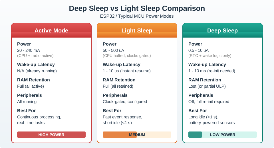
Use the comparison as a review prompt. A device that samples once per hour can usually afford a cold wake, rebuild state, and pay the boot cost. A device that wakes every few seconds to debounce a button, watch a threshold, or maintain a short receive window may spend more charge repeatedly restarting than it would have spent staying in a lighter retained mode. The correct choice is the mode with the lowest measured charge over the whole interval, including state restore, sensor settling, clock startup, bus configuration, and radio rejoin.
Intuition only: pick the sleep mode by comparing the current saved during sleep against the extra energy spent waking from it. Short naps favor a light mode; long sleeps favor a deep one.
What Each Mode Trades
Sleep current
Deeper modes draw less, from milliamps in light sleep down to microamps in deep sleep.
Retention
Light sleep keeps RAM and peripherals; deep sleep keeps almost nothing, so state must be rebuilt.
Wake cost
A deeper mode costs more energy and time to wake, because it must reboot and re-initialize.
Peripheral rails
Whatever you leave powered during sleep adds to the floor regardless of the processor mode.
Overview Knowledge Check
6.22 Find The Sleep-Depth Break-Even
Compare the two modes over a sleep interval T. Light sleep costs about Ilight x T. Deep sleep costs Ideep x T plus a fixed wake energy Ewake for the reboot. Deep sleep wins only when its lower floor has had enough time to repay the wake cost.
Worked Example: Light Sleep Versus Deep Sleep
Light sleep draws 0.8 mA with a negligible wake. Deep sleep draws 10 uA but needs a 250 ms boot at 40 mA, so Ewake = 40 mA x 0.25 s = 10 mA-s. Setting the two equal: 0.010 x T + 10 = 0.8 x T gives T = 10 / 0.79 = 12.7 s.
- Wake every 5 s: light = 0.8 x 5 = 4.0 mA-s; deep = 0.010 x 5 + 10 = 10.05 mA-s. Light sleep wins by about 2.5x.
- Wake every 60 s: light = 0.8 x 60 = 48 mA-s; deep = 0.010 x 60 + 10 = 10.6 mA-s. Deep sleep wins by about 4.5x.
- Break-even: near 13 s. Below it, the boot overhead makes deep sleep more expensive; above it, the low floor pays off.
Then handle the peripherals. A sensor drawing 1 mA left powered through a 60 s sleep leaks 1 x 60 = 60 mA-s per cycle - a hundred times the 0.6 mA-s the processor's deep sleep uses. Power-gating that sensor, at the cost of a small re-power and settle on wake (say 2 mA for 20 ms, 0.04 mA-s), removes almost all of that leak.
Sleep Strategy Ledger
Practitioner Knowledge Check
6.23 Hidden Leakage Paths Defeat Power Gating
Power-gating a peripheral only helps if you cut every path into it. A classic trap involves the I2C bus. Suppose you switch off a sensor's power rail to save its 1 mA during sleep, but leave the bus pull-up resistors powered and the I2C lines high. Current then flows from the pull-ups through the sensor's input protection diodes into the now-unpowered chip. That leak both wastes current and can partially power the sensor through its own pins, so the gated device is neither fully off nor properly saving energy.
The same pattern hides in other places: a peripheral clock left enabled keeps a block toggling, a GPIO left driving into a depowered load pushes current through protection structures, and a floating input can oscillate and draw switching current. The fixes are specific and cheap. Before sleeping, drive shared bus lines low or gate the pull-ups on the same switch as the sensor, disable unused peripheral clocks, and set unused pins to a defined low-leakage state. The rule is to power-gate the whole island - rail, pull-ups, and signals together - not just the chip's main supply pin.
Put a number on the hidden path before dismissing it. A 4.7 kOhm pull-up on a 3.3 V bus can source about 3.3 / 4700 = 0.70 mA if a depowered input clamps the line low through a diode path. Two lines can therefore create a milliamp-scale leak, larger than many MCU deep-sleep currents by two orders of magnitude. Even a partial 0.2 mA leak on each line for a 60 s sleep interval adds 0.4 x 60 = 24 mA-s, which dwarfs the 0.6 mA-s of a 10 uA processor sleep over the same interval. The measurement proof is simple: change the bus state, gate the pull-ups with the sensor rail, and confirm the sleep floor falls in the full-cycle trace.
Leakage Paths To Close Before Sleep
Pull-ups into gated chips
Bus pull-ups feed current through protection diodes into a depowered sensor. Gate them with the rail or drive lines low.
Enabled clocks
An unused peripheral clock keeps a block switching. Disable clocks for anything not in use during sleep.
Driven-into loads
A GPIO held high into a depowered device leaks through its pins. Set outputs to a safe low-leakage level first.
Floating inputs
An undriven input can oscillate and draw switching current. Tie unused inputs to a defined level.
Under-the-Hood Knowledge Check
6.24 Summary
This chapter covers low-power strategies including sleep-mode selection, duty-cycle policy, peripheral power gating, firmware timing discipline, radio batching, and voltage or clock scaling.
6.25 Key Takeaway
In the field, optimize charge per useful outcome. Sleep modes, power gating, batching, retry limits, and firmware timing should be selected from measured traces and failure-mode requirements.