17 Power Management Tools
Battery-Life Calculators, Sensitivity Sweeps, and Measurement Validation
17.1 Start With a Calculator You Do Not Trust Yet
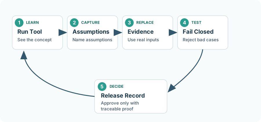
A battery-life calculator can make a design look precise even when the inputs are guesses. Treat every tool result as a hypothesis: useful for sensitivity, unsafe as proof until measurements agree.
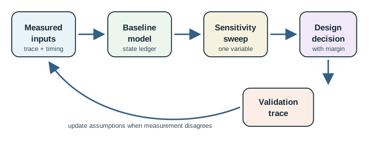
The simple workflow is measure, model, sweep, interpret, then return to the bench for the inputs that move the answer most.
17.2 Power Management Tools
Interactive calculators can speed up IoT energy design, but only if their inputs match the device being built. A calculator cannot know the leakage of your board, the retry pattern of your radio, the cutoff voltage of your regulator, or the temperature range of the deployment unless you enter those values deliberately.
This chapter treats calculators as decision-support tools, not proof. The workflow is: measure inputs, model the energy ledger, run sensitivity sweeps, make a design change, and validate the result with traces.
17.3 Learning Objectives
By the end of this chapter, you will be able to:
- Select the right power-management tool for a design question.
- Prepare measured inputs before running a battery-life estimate.
- Build a power-state ledger from active, transmit, receive, idle, and sleep intervals.
- Run sensitivity sweeps without changing several assumptions at once.
- Interpret tool outputs as ranges, constraints, and evidence gaps.
- Validate calculator results against bench measurements and field logs.
- Recognize unrealistic lifetime, solar, protocol, and fleet-maintenance claims.
- A calculator result is only as good as its inputs.
- Use measured whole-device current when possible, not isolated component datasheet values.
- Battery capacity must be derated for usable voltage range, temperature, age, pulse load, and self-discharge.
- Sensitivity sweeps are more useful than a single lifetime number.
- A tool output should create a test plan: what to measure next, what assumption is risky, and what margin remains.
17.4 Tool Workflow
The useful path through an energy tool starts before the calculator opens.
17.4.1 1. Measure
Capture whole-device current for each power state. Include regulator losses, sensors, pull-ups, LEDs, radio retries, and board leakage.
17.4.2 2. Model
Enter the state currents, durations, wake interval, usable capacity, and operating limits. Keep the first model simple enough to audit.
17.4.3 3. Sweep
Change one variable at a time: sleep current, transmit interval, payload size, retry rate, sensor warm-up time, or usable capacity.
17.4.4 4. Validate
Compare predicted average current with a power trace. If they disagree, fix the model before using it for lifetime or sourcing decisions.
17.5 Choose the Right Tool
Different questions need different tool types. Do not use a fleet cost calculator when the open question is still “what current does this board actually draw?”
17.5.1 Battery-Life Estimator
Use when the power states are known and the question is whether a usable battery capacity can meet a lifetime target.
Input quality gate: measured average current or measured state currents plus timing.
17.5.2 Power-State Ledger
Use when the device has several modes and you need to see which state dominates the energy budget.
Input quality gate: current, duration, and event count for every state in one reporting period.
17.5.3 Sensitivity Sweep
Use when a design misses its target and you need to know which change has the largest effect.
Input quality gate: one baseline model, one varied parameter, and a recorded output range.
17.5.4 Protocol Comparator
Use when comparing radio options for the same payload, coverage, latency, and reliability need.
Input quality gate: complete exchange time, acknowledgments, receive windows, retries, and join or association costs.
17.5.5 Harvesting Sizer
Use when checking whether measured source energy can support a measured load through weak-source intervals.
Input quality gate: local source survey, converter efficiency, storage leakage, and autonomy requirement.
17.5.6 Validation Notebook
Use when turning the calculator into a repeatable engineering record.
Input quality gate: tool version, assumptions, raw trace files, model inputs, output ranges, and decision notes.
17.6 Inputs Before Outputs
The best improvement to a power calculator is usually better input evidence.
Input
Use In Tool
Common Failure
Evidence To Keep
State current
Active, TX, RX, sensor warm-up, idle, and sleep current values.
Using datasheet typical values for a full board.
Power trace screenshots, meter settings, firmware state labels.
State duration
Seconds or milliseconds spent in each state per cycle.
Ignoring retries, startup time, or receive windows.
Trace markers, logs, packet captures, timing notes.
Usable capacity
Capacity after cutoff voltage, temperature, age, pulse load, and reserve.
Entering nominal battery capacity as fully usable energy.
Battery datasheet, cutoff policy, derating rationale.
Deployment rule
Reporting interval, latency target, outage tolerance, and maintenance policy.
Optimizing lifetime while violating service requirements.
Requirement record and acceptance threshold.
17.7 Battery-Life Ledger
A calculator should expose the ledger behind the lifetime number. For one reporting period:
\[ I_{avg} = \frac{I_{active}t_{active} + I_{tx}t_{tx} + I_{rx}t_{rx} + I_{sleep}t_{sleep}}{t_{period}} \]
Then:
\[ life_{hours} = \frac{usable\ battery\ capacity_{mAh}}{I_{avg,mA}} \]
A field sensor wakes every 15 minutes. The measured trace shows 8 mA active for 2.0 s, 42 mA transmit for 0.8 s, and 12 uA sleep for the rest of the 900 s period.
- Active charge:
8 mA x 2.0 s = 16 mA*s - Transmit charge:
42 mA x 0.8 s = 33.6 mA*s - Sleep charge:
0.012 mA x 897.2 s = 10.8 mA*s - Average current:
(16 + 33.6 + 10.8) / 900 = 0.067 mA - With 1500 mAh usable capacity, first-pass lifetime is about 2.6 years.
That number is not a promise. It becomes useful when the same firmware is measured again after design changes and when field logs confirm retry behavior.
17.8 Sensitivity Sweeps
A sensitivity sweep answers “what should we optimize first?” It is usually more useful than arguing about a single predicted lifetime.
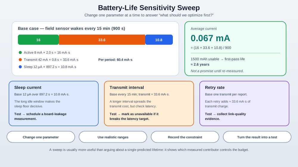
Change one parameter Hold every other assumption fixed. Otherwise the sweep cannot tell you which change mattered.
Use realistic ranges Sweep values the firmware and hardware can actually support, not fantasy deep-sleep or zero-retry numbers.
Record the constraint If a longer report interval saves energy but breaks latency, mark it as unavailable rather than “best.”
Turn the result into a test If sleep current dominates, schedule a board-leakage measurement. If retries dominate, collect link-quality evidence.
17.9 Interpreting Tool Outputs
Treat the output as a decision record:
- Dominant consumer: which state or event controls the energy budget?
- Margin: how far is the result from the target after derating?
- Assumption risk: which input was guessed instead of measured?
- Constraint failure: did the energy-saving option break latency, range, sample quality, or maintenance policy?
- Next measurement: what trace, field log, or datasheet limit would most reduce uncertainty?
Be skeptical when a tool reports “infinite” battery life, perpetual solar operation, exact multi-year lifetime, or large fleet savings without showing battery derating, self-discharge, field temperature, retry behavior, maintenance access, and measured current traces.
17.10 Validation Loop
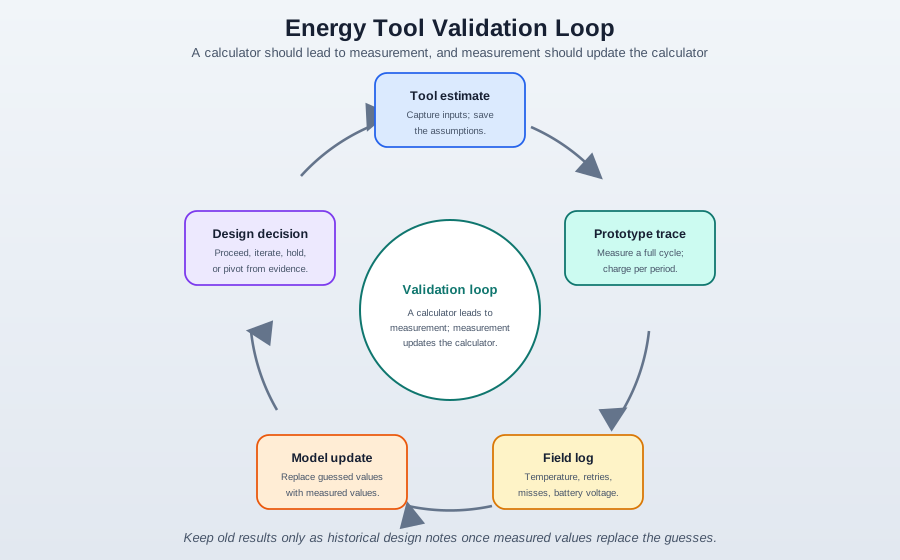
A calculator should lead to measurement, and measurement should update the calculator.
17.10.1 Tool Estimate
Capture input values and output range. Save the assumptions next to the result so another reviewer can reproduce it.
17.10.2 Prototype Trace
Measure a complete reporting cycle. Compare predicted and measured charge per period, not only peak current.
17.10.3 Field Log
Check temperature, retries, missed reports, battery voltage, and charging or harvesting events after deployment.
17.10.4 Model Update
Replace guessed values with measured values. Keep old results only as historical design notes.
17.11 Example Review Flow
Suppose a soil sensor must report every 15 minutes for at least two years.
- Measure the first firmware trace and build the state ledger.
- Enter usable capacity, not nominal capacity.
- Run a sensitivity sweep for sleep current, transmit duration, and retry count.
- Discover that radio retries control the lifetime range more than sensor current.
- Test antenna placement and spreading-factor settings before changing the battery.
- Re-measure the full cycle and update the calculator with the new trace.
- Record the final margin and the field conditions where it is valid.
The tool helps because it focuses the next experiment. It does not replace the experiment.
17.12 Tool Review Checklist
Inputs are trace-backed Every major current or duration value points to a bench trace, packet log, or controlled measurement.
Capacity is usable Battery capacity reflects voltage cutoff, temperature, age, pulse limits, self-discharge, and reserved margin.
Protocol cost is complete The model includes association, acknowledgments, receive windows, retries, and failed transmissions when relevant.
Output is a range The design record shows best-case, expected, and conservative estimates, not a single polished number.
Decision is explicit The result says what changed: interval, firmware mode, radio policy, battery choice, storage size, or measurement plan.
Validation is scheduled The next bench or field check is named before the design is treated as accepted.
17.13 Common Pitfalls
Datasheets describe components under test conditions. A real board includes regulators, sensors, leakage paths, firmware timing, pull-ups, LEDs, and radio behavior that can change the average current substantially.
If the radio or sleep leakage dominates the ledger, replacing a small sensor load will not move the lifetime enough to justify the effort.
A protocol comparison is only fair when payload size, range, latency, reliability, network availability, and retry behavior are comparable.
Harvesting tools need measured source power, converter behavior, storage leakage, autonomy, and weak-source periods. A bright-day estimate does not prove energy-neutral operation.
If the model inputs, tool version, trace files, and decision notes are not saved, the result cannot be audited when the hardware or firmware changes.
17.14 Check Your Understanding
17.15 Knowledge Check: Trusting A Calculator
17.16 Match Tools To Questions
17.17 Order The Review Workflow
17.18 Label The Tool Loop
17.20 What’s Next
Review the full learning path and where tool-supported analysis fits.
Connect usable capacity and storage behavior to calculator inputs.
Case Studies and Best Practices
Evaluate real design decisions using the same evidence-first tool workflow.
17.21 A Calculator’s Job Is To Show Sensitivity, Not Just A Number
A battery-life tool turns a state ledger into a single number, but that number is the least useful thing it produces. The valuable output is the sensitivity: which input, if you changed it, would move the lifetime the most. For a duty-cycled device the model is Iavg = Isleep + (Iactive - Isleep) x D, where D is the duty cycle. Depending on D, either the sleep term or the active term dominates, and the tool's job is to tell you which.
For infrequent reporters - a device that wakes for a fraction of a second every few minutes or hours - the duty cycle is tiny, so the sleep current term carries most of the average. That is why sleep current so often decides battery life: not because it is large, but because it runs almost all the time.
Make the sensitivity concrete before optimizing. If the estimate is 1000 mAh / 26.9 uA = 37,175 h, or about 4.2 years, a 5 uA error in sleep current changes the average to 31.9 uA and shortens life to about 3.6 years. Both figures are ideal, device-only lifetimes: they ignore the cell's own self-discharge, which for this size of cell is a fixed current comparable to the device's own average and roughly halves the realistic life to about 2.1 years (worked out below). The same 5 uA error in a short active pulse is usually invisible because it is multiplied by only a tiny duty cycle. The calculator is therefore useful when it ranks which assumption deserves measurement first.
Intuition only: a lifetime number without a sensitivity sweep can point you at the wrong optimization. Always ask the tool which input the answer depends on before trying to improve it.
What A Good Tool Reveals
Average current
The weighted blend of sleep and active current that sets the whole estimate.
Dominant term
Whether sleep or active carries most of the average, which depends on the duty cycle.
Sensitivity
How much the lifetime moves when each input changes, so effort goes to the steepest input.
Input trust
Which inputs are measured versus guessed, since the most sensitive input must be the best measured.
Overview Knowledge Check

Phoebe’s Why
This page’s own baseline – 1000 mAh divided by 26.9 µA, about 4.2 years – treats the cell as a pure charge reservoir that only the device drains. Every real cell also drains itself, and that self-discharge current does not care what the device is doing; it is a floor under the total average current, not a slice of the device’s own budget. This page’s warning to “be skeptical when a tool reports… perpetual solar operation… without showing battery derating [and] self-discharge” is exactly right, and its own 26.9 µA example is small enough that a typical self-discharge current sits right on top of it – close enough to change the headline number, not just the decimal places.
The Derivation
The calculator’s own model already used by this page, now with the leak the ledger omitted added back in:
\[I_{total} = I_{device,avg} + I_{sd}, \qquad \mathrm{Life} = \frac{C_0}{I_{total}}\]
The marginal value of shaving device current further – the sensitivity this page’s tool is built to expose – is the derivative of that same expression:
\[\frac{\partial\,\mathrm{Life}}{\partial\,I_{device}} = -\frac{C_0}{I_{total}^{\,2}}\]
which shrinks fast once \(I_{sd}\) stops being negligible next to \(I_{device}\).
Worked Numbers: This Page’s Own 1000 mAh, 26.9 µA Baseline
- The leak, sized the same way as elsewhere on this site: a catalog-typical \(2.00\%\)/month Li-ion self-discharge on a \(1000\) mAh cell is \(I_{sd}=(0.02\times1000)/720\ \text{h}=0.0278\) mA \(=27.8\ \mu\text{A}\) – larger than this page’s own \(26.9\ \mu\text{A}\) measured device average.
- Corrected life: \(I_{total}=26.9+27.8=54.7\ \mu\text{A}\), so \(\mathrm{Life}=1000/0.0547=18{,}289\) h \(=2.09\) years – barely half of this page’s own stated \(4.2\)-year headline, purely from a term the sensitivity sweep never included as an input.
- What that does to the sensitivity itself: the marginal value of trimming one more µA of device current is \(\propto1/I_{total}^2\). At the device-only baseline that derivative is worth about \(1382\) h per µA; once self-discharge is folded in, it is worth only about \(334\) h per µA – a \(4.1\times\) drop, meaning every hour spent chasing sub-µA sleep-current improvements is worth barely a quarter of what the naive sweep implies.
- The lesson for the tool, not just the number: this page is right that a sensitivity sweep beats a single lifetime figure, but the sweep is only as complete as its input list – self-discharge belongs on it as its own fixed-current row, not folded silently into “derating.”
17.22 Sweep Each Input; The Steepest One Wins
To find where optimization pays, halve one input at a time and read the new lifetime. The input whose halving moves the lifetime most is the one to work on. For infrequent reporters, that is almost always the sleep current.
Worked Example: Report Once Per Hour
The node wakes for a 50 mA burst lasting 0.5 s once every 3600 s and sleeps at 20 uA otherwise.
- Baseline: active 50 mA x 0.5 s = 25 mA-s; sleep 0.020 mA x 3599.5 s = 72 mA-s; total 97 mA-s per hour, so Iavg = 26.9 uA. Sleep is 74% of the budget. On a 1000 mAh cell that is about 4.2 years, ideal and device-only (no self-discharge -- see the correction above, which roughly halves it to about 2.1 years realistically).
- Halve the sleep current (20 to 10 uA): sleep charge falls to 36 mA-s; total 61 mA-s; Iavg = 16.9 uA; life about 6.7 years. That is +59%.
- Halve the active current (50 to 25 mA): active charge falls to 12.5 mA-s; total 84.5 mA-s; Iavg = 23.5 uA; life about 4.9 years. That is only +15%.
Halving sleep adds roughly two and a half years; halving the far larger active current adds barely half a year. The steep input is sleep, because at this duty cycle it dominates the average. A tool that showed only the baseline 4.2-year number would not have told you that.
Use the same sweep to set a measurement plan. The 20 uA sleep term contributes 72 / 97 = 74% of the hourly charge, so it should be measured across the real board's regulator, pull-ups, sensors, and interface chips. The 50 mA active pulse contributes 25 / 97 = 26%; it still matters, but reducing it is a second-pass optimization unless the reporting interval changes.
Sensitivity Sweep Ledger
All lifetimes in this ledger are ideal, device-only figures used to compare the relative sensitivity of sleep versus active current; none include the cell's own self-discharge, which realistically roughly halves the baseline to about 2.1 years (see the correction above).
Practitioner Knowledge Check
17.23 The Most Sensitive Input Deserves The Most Measurement
Because lifetime is inversely proportional to average current, a percentage error in the dominant current becomes almost the same percentage error in the predicted lifetime. That makes the most sensitive input the most dangerous one to guess. For the hourly reporter above, sleep current is the dominant term, so feeding the tool a datasheet sleep figure instead of a measured one can wreck the estimate.
Suppose the datasheet promises 10 uA deep sleep and the tool predicts about 6.7 years, but the assembled board actually sleeps at 200 uA because of a regulator and interface chip. The real average becomes about 207 uA and the true life is roughly 0.55 years - the tool overstated lifetime by more than twelvefold, entirely from one wrong input in the term the answer was most sensitive to. The lesson is procedural: run the sweep first, find the dominant input, and spend your measurement effort there. A carefully measured active current paired with a guessed sleep current is precision on the wrong number. The regime also matters: if the same node reported every few seconds, the active term would dominate instead, and the measurement priority would flip.
The inverse relationship also explains why optimistic capacity and optimistic current errors multiply. If a coin cell is entered as 1000 mAh instead of a realistic 650 mAh at the deployment temperature, and the dominant sleep current is entered as 10 uA instead of 200 uA, the model is wrong on both numerator and denominator. The ratio is roughly (1000 / 650) x (200 / 10) = 30.8, so a multi-year prediction can collapse to weeks. Good tools force those assumptions into visible fields instead of hiding them behind a single lifetime output.
Turning Sensitivity Into Practice
Garbage in
A wrong value in the dominant term propagates almost one-to-one into the lifetime estimate.
Measure the dominant term
Whichever input the sweep marks steepest is the one to measure on real hardware, not read from a datasheet.
Regime awareness
Frequent reporting shifts dominance to active current; rerun the sweep when the duty cycle changes.
Report ranges
Show expected and conservative lifetimes, since a single figure hides the sensitivity to uncertain inputs.
Under-the-Hood Knowledge Check
17.24 Summary
This chapter uses interactive tools and calculators to explore battery life, duty cycle, communication cost, harvesting assumptions, and optimization tradeoffs.
17.25 Key Takeaway
Interactive tools are useful because they expose assumptions. Change duty cycle, current, radio sessions, battery capacity, and harvesting input, then verify the result with measurements before using it for design.