7 Energy Measurement and Profiling
Current Traces, Shunt Selection, Duty-Cycle Evidence, and Battery-Life Validation
7.1 Start With the Trace, Not the Datasheet
Datasheets tell you what a part can do under stated conditions; the current trace tells you what your assembled device actually did. Both matter, but only the trace can prove the budget.
This chapter follows the measurement loop: predict the state budget, capture it with the right instrument, explain mismatches, then keep the evidence with the design decision.
Battery Bruno
“A budget on a spreadsheet is a guess — the trace is the only thing that gets to call it a fact.”
Here Bruno picks the tool for the pulse he’s chasing and reads a bad trace for what it’s really telling him.

Phoebe’s Why
This chapter is right that a shunt resistor perturbs the very rail it is measuring, and its own arithmetic already shows a 1 ohm shunt stealing 200 mV during a 200 mA pulse. But a coin cell’s internal resistance forms the exact same kind of divider with the load, in series with whatever the meter adds – and a coin cell’s internal resistance is not small. Its tiny electrode area cannot deliver current the way a full-size cylindrical cell can, so its own resistance often dwarfs the shunt sitting in series with it. That reframes the chapter’s own coin-cell warning: the instrument’s 200 mV perturbation is real, but for many coin-cell pulse currents the cell would sag itself into brownout territory with a perfect, zero-burden ammeter in the circuit. The measurement discipline this chapter teaches is still necessary – it just is not sufficient to rescue a design that is already asking more of the cell than its own chemistry can deliver.
The Derivation
The cell’s internal resistance and the instrument’s shunt sit in series with the same pulse current, so their voltage drops add directly:
\[V_{term} = V_{oc} - I\,(R_{int} + R_{shunt})\]
The instrument’s own contribution is exactly the burden-voltage relationship already used above:
\[\Delta V_{shunt} = I \times R_{shunt}\]
so the cell’s native, instrument-free sag is the same Ohm’s-law form applied to \(R_{int}\) alone:
\[\Delta V_{cell} = I \times R_{int}\]
Worked Numbers: This Chapter’s Own 200 mA Pulse
- The chapter’s own instrument perturbation: \(\Delta V_{shunt}=0.200\times1=0.200\) V (matches the “200 mV” already stated above).
- The coin cell’s own native sag (catalog-typical fresh CR2032 internal resistance, \(R_{int}\approx10\ \Omega\); datasheets commonly show it climbing into the tens of ohms as the cell depletes or runs cold): \(\Delta V_{cell}=0.200\times10=2.00\) V. On this chapter’s own “partly discharged 3.0 V system,” that alone leaves only about \(1.00\) V at the load – already a likely brownout before the meter is even connected.
- With the meter in circuit: \(\Delta V_{total}=0.200\times(10+1)=2.20\) V, terminal \(\approx0.80\) V. The instrument’s marginal share of that drop is \(2.20-2.00=0.200\) V – real, and worth removing, but only about a tenth of the total sag.
- The honest conclusion: for this chapter’s own coin-cell scenario, a lower-burden shunt improves the measurement’s accuracy, but it does not rescue the design. The dominant term is \(I\times R_{int}\), which belongs to the cell, not the meter – the charge-versus-energy question this chapter flags (“still needs battery derating, temperature effects, self-discharge, and reserve margin,” worked in full in Energy-Aware Introduction) governs whether the average 312 uA lasts 256 days, but it is this instantaneous \(I\times R_{int}\) sag that decides whether a single 200 mA radio burst survives at all.
7.2 Energy Measurement and Profiling
A low-power design is not finished when the spreadsheet looks good. It is finished when the hardware, firmware, sensors, radio, regulator, and debug path have been measured together under realistic operating conditions.
This chapter focuses on practical measurement: choosing the right instrument, sizing a shunt without disturbing the device, capturing a full current trace, explaining anomalies, and converting the trace into an average-current estimate that can be tested again after each fix.
7.3 Learning Objectives
By the end of this chapter, you will be able to:
- Choose a measurement method for sleep current, active current, radio bursts, and startup transients.
- Explain burden voltage, shunt power, dynamic range, and why one fixed shunt often cannot cover the whole profile.
- Build a repeatable measurement setup that isolates the target device from USB, LEDs, debug adapters, and regulator leakage.
- Capture a full duty-cycle trace and connect current spikes to firmware states.
- Calculate average current from measured state charge and use it to update battery-life estimates.
- Identify common measurement mistakes before they turn into false optimization work.
- Measure the complete product rail, not only the MCU, when estimating deployed battery life.
- Measure the isolated target rail, not the USB input of a development board, when validating sleep current.
- A multimeter can check steady current, but it usually misses short radio, sensor, and wakeup pulses.
- A shunt resistor creates voltage drop; too much drop changes the circuit you are trying to measure.
- Battery-life estimates should come from measured charge per cycle, not from a single datasheet sleep-current number.
- First you define the measurement question and decide whether the target is sleep current, state cost, battery survival, or before/after improvement.
- Then you choose the measurement chain, including shunt value, burden voltage, dynamic range, and instrument bandwidth.
- Next you capture the full duty-cycle trace and mark firmware phases so each current region has a cause.
- Finally you turn charge per cycle into a battery-life estimate, then use the quizzes and shunt deep dives to check the setup itself.
Checkpoints recap the practical rule; “Deep dive” and collapsed warnings are optional on a first read.
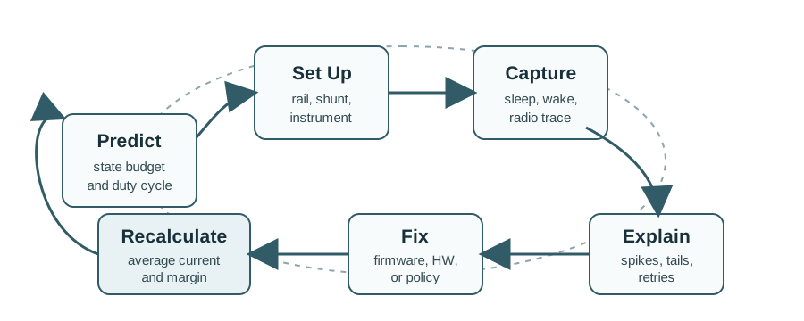
7.4 Measurement Evidence Loop
Good energy profiling is an iterative loop. The first trace rarely confirms the original model; it usually reveals hidden loads, extra wake time, radio retries, or a board path that was not in the spreadsheet.
7.4.1 Predict
List each state, expected current, expected duration, and wake frequency before measuring. The prediction gives the trace something concrete to confirm or reject.
7.4.2 Capture
Record the whole product rail during sleep, wake, sensing, processing, radio work, and return to sleep. A partial trace hides duty-cycle mistakes.
7.4.3 Explain
Tie every visible current region to firmware, hardware, or radio behavior. Unexplained spikes are defects until proven otherwise.
7.4.4 Recalculate
Update the average current and battery-life estimate from measured charge per cycle, then repeat after each fix.
Checkpoint: Measurement Question
You now know:
- Sleep validation, state-cost diagnosis, battery survival, and before/after fixes require different measurement points.
- The evidence loop is predict, capture, explain, recalculate, and repeat with a complete duty-cycle trace.
7.5 What to Measure
The measurement target depends on the question you are answering.
7.6 Current Measurement Chain
Most IoT current measurements place a known impedance in series with the device supply and measure the voltage across that impedance. The instrument may be a multimeter, oscilloscope, current-sense amplifier, auto-ranging power profiler, or source-measure unit.
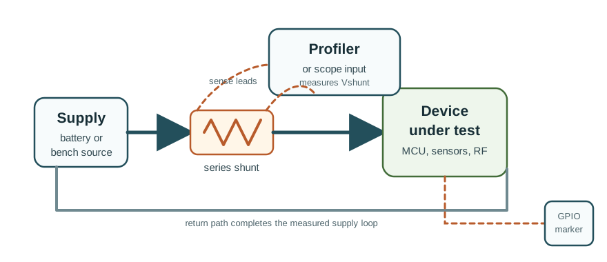
The basic relationship is:
\[I = \frac{V_{shunt}}{R_{shunt}}\]
The design constraint is burden voltage:
\[V_{burden} = I_{max} \times R_{shunt}\]
If the burden voltage is too high, the device sees a lower supply voltage and may behave differently. For example, a 100 ohm shunt gives useful resolution at 10 uA, but it would drop 5 V at 50 mA. That does not measure the device; it prevents the device from operating normally.
For a sensor that sleeps at 10 uA and wakes at 50 mA:
- To produce at least 1 mV at 10 uA, the shunt must be at least 100 ohm.
- To keep burden voltage below 100 mV at 50 mA, the shunt must be at most 2 ohm.
- One fixed shunt cannot satisfy both constraints.
Use switchable shunts, an auto-ranging profiler, or separate steady-state and transient measurements.
Checkpoint: Shunt Tradeoff
You now know:
- The current comes from Ohm’s law:
I = V_shunt / R_shunt. - One fixed shunt may not span 10 uA sleep and 50 mA wake current without changing the device under test.
7.7 Tool Selection
Tool choice is about current range, time resolution, burden voltage, and repeatability. Avoid choosing a tool only because it is convenient.
Bruno’s Power Budget
- Draw: a multimeter reads steady current fine but blinks right past a millisecond radio burst.
- Sleep: an auto-ranging profiler is the one tool built to span sleep-to-radio dynamic range without a manual switch.
- Life: pick the instrument for the pulse you need to catch, not the one already sitting on the bench.
7.8 Capturing a Power Profile
A useful current trace should show the entire cycle: sleep baseline, wake, sensor stabilization, data acquisition, processing, radio activity, shutdown, and return to sleep. The trace is only useful if every region can be explained.
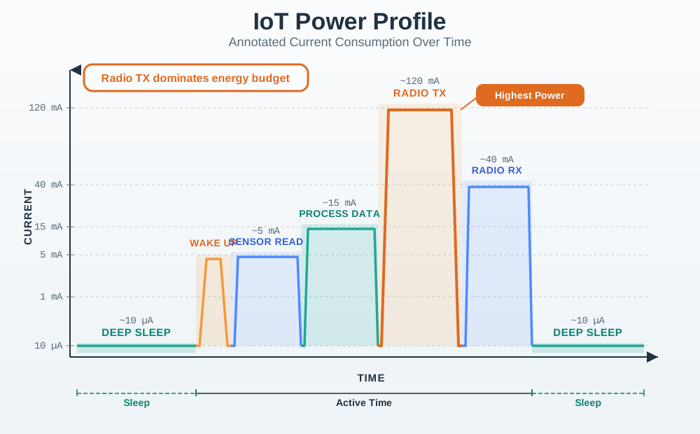
Capture enough cycles One clean cycle can be misleading. Capture multiple cycles so background timers, retries, maintenance tasks, and sensor warm-up variation can appear.
Mark firmware phases Toggle a spare GPIO at state boundaries so the current trace can be aligned with code paths.
Preserve the supply condition Measure at the voltage the product will actually see, including the lowest expected battery voltage.
Record the context Save firmware build, reporting interval, radio configuration, sensor load, supply voltage, temperature, and instrument range settings with the trace.
7.9 Firmware Markers
The trace shows when current changed; the marker tells you which code path changed it.
GPIO markers help connect a waveform to a firmware state without guessing. The marker pin should be measured on a logic input or scope channel; it should not drive a load that changes the power profile.
// Pseudocode: use a spare pin only as a timing marker.
void sample_and_report(void) {
    profile_marker_high();   // wake and sensor phase starts
    power_sensor_on();
    wait_for_sensor_to_settle();
    read_sensor();
    profile_marker_low();    // sensor phase ends

    profile_marker_high();   // communication phase starts
    radio_send_packet();
    radio_shutdown();
    profile_marker_low();    // communication phase ends

    enter_sleep();
}
Use markers sparingly. Too many markers clutter the trace, and marker code must not keep clocks, debug modules, or peripherals awake longer than production firmware.
Checkpoint: Trace Interpretation
You now know:
- A useful trace includes sleep baseline, wake, sensor stabilization, data acquisition, processing, radio activity, shutdown, and return to sleep.
- Multiple cycles plus GPIO markers reveal retries, maintenance tasks, timers, and code phases that one clean cycle can hide.
7.10 From Trace to Battery-Life Estimate
The most useful output of profiling is charge per useful cycle. For each region:
\[Q_{state} = I_{state} \times t_{state}\]
Then:
\[I_{avg} = \frac{\sum Q_{state}}{T_{cycle}}\]
For a 10-minute environmental monitor:
Total charge per cycle is about 52 uAh. Because the cycle is one sixth of an hour, the measured average current is about 312 uA. A 2400 mAh cell with 80% usable capacity would be estimated at roughly 256 days before adding battery derating, temperature effects, self-discharge, and reserve margin.
The point is not the exact number. The point is that the radio event dominates the measured charge, so the next engineering step should be radio timing and retry reduction, not micro-optimizing a short CPU calculation.
Checkpoint: Lifetime Evidence
You now know:
- Charge per useful cycle is the evidence that connects a current trace to a battery-life estimate.
- In the 10-minute example, the radio event contributes 46.7 uAh out of about 52 uAh, so it dominates the average.
- The rough 256-day estimate still needs battery derating, temperature effects, self-discharge, and reserve margin.
7.11 Common Findings and Fixes
Now the estimate has pointed at the dominant cost; next, decide whether the symptom comes from hardware, firmware, radio behavior, or the setup.
Bruno’s Power Budget
- Draw: sleep current far above budget usually traces to an LED, USB bridge, or regulator quiescent draw, not the MCU.
- Sleep: an unexpected periodic pulse during sleep is a timer, watchdog, or background task – found by disabling suspects one at a time.
- Life: a slow return-to-sleep tail often means a shutdown sequence never actually finished.
7.12 Validation Conditions
A single room-temperature bench trace is useful, but it is not final validation. Repeat the measurement under the conditions that can change energy behavior.
- Final hardware: development boards include loads that production hardware may not have, and production boards include leakage paths that prototypes may hide.
- Battery voltage range: radio transmit current, regulator efficiency, brownout margin, and sensor behavior can change as voltage falls.
- Temperature range: leakage, battery capacity, sensor settling, and oscillator behavior can shift at temperature extremes.
- Real radio conditions: weak signal, interference, acknowledgments, retries, receive windows, and connection setup can dominate the energy budget.
- Real sensor load: wet probes, long cables, external pull-ups, and slow stabilization can extend active time.
- Multiple units: one good board does not prove a manufacturing population.
Do not treat profiling as a final demo. Profile early enough that the design can still change: regulator choice, antenna placement, sensor power gating, firmware wake policy, and reporting interval all become expensive to change late.
7.13 Check Your Understanding
7.14 Knowledge Check: Measurement Point
7.15 Knowledge Check: Shunt Burden
7.16 Matching Quiz: Measurement Method to Use Case
7.17 Ordering Quiz: Repeatable Profiling Workflow
7.18 Label the Measurement Setup
7.19 One Shunt Cannot See Both Sleep And Transmit
Measuring a device's current usually means putting a small resistor - a shunt - in series and reading the voltage across it, since V = I x R. That voltage is called the burden voltage, and it is subtracted from the supply the device actually receives. The whole craft of current measurement is choosing a shunt that produces a readable voltage without stealing so much that it disturbs the device.
The hard part is dynamic range. An IoT node might sleep at 10 uA and transmit at 200 mA, a ratio of 20000 to 1. A single fixed shunt cannot serve both ends: a value large enough to make 10 uA readable would drop a device-killing voltage at 200 mA, while a value small enough to be harmless at 200 mA would produce an unreadable signal at 10 uA. That tension is why serious current measurement uses auto-ranging instruments.
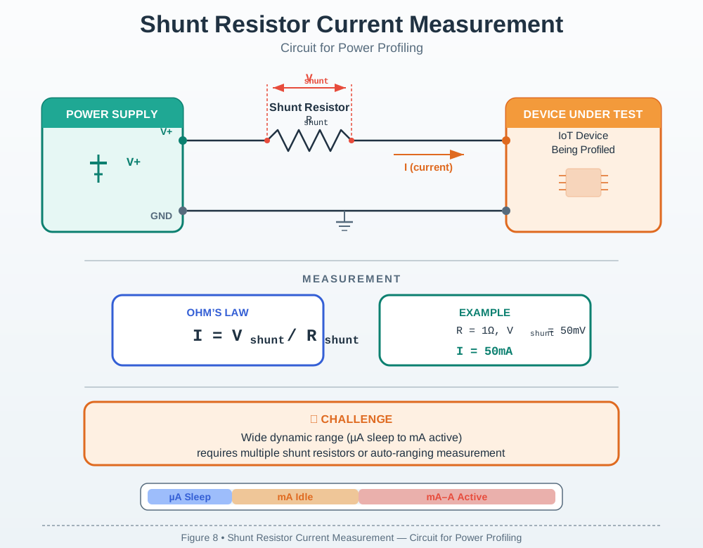
Use the circuit as a setup checklist before trusting a trace. The supply, shunt, sense leads, and device must form one intentional measurement loop; measuring the wrong side of a regulator, USB bridge, or debug adapter changes the question. Record the shunt value and the maximum observed shunt voltage with every capture. For example, a 0.25 ohm shunt at 200 mA drops 50 mV, which may be acceptable; a 10 ohm shunt at the same peak drops 2 V and turns the measurement into a brownout test.
Intuition only: the shunt must be small enough not to disturb the peak current and large enough to resolve the sleep current. Those two demands usually cannot be met by one resistor, so the range must switch.
The Measurement Chain
Shunt resistor
Converts current to a voltage by Ohm's law. Its value trades resolution against burden.
Burden voltage
The drop the shunt steals from the supply. Too large and it changes the device's behavior.
Dynamic range
The sleep-to-peak current ratio, often tens of thousands to one, that one fixed shunt cannot span.
Bandwidth
How fast the chain can follow a transient. Too slow and it averages away the peaks.
Overview Knowledge Check
7.20 Size The Shunt For Burden Versus Resolution
Two inequalities bound the shunt. The burden limit keeps the peak drop small: R <= V_burden_max / I_peak. The resolution limit keeps the sleep signal readable above the amplifier's noise and offset: R >= V_min / I_sleep. When these two bounds cross, no single value works.
Worked Example: A Node From 10 uA To 200 mA
Target a burden under 50 mV at the 200 mA peak and a readable 100 uV minimum at the 10 uA sleep.
- Burden limit: R <= 0.050 V / 0.200 A = 0.25 ohm. The shunt must be no larger than a quarter ohm.
- Resolution limit: R >= 100 uV / 10 uA = 10 ohm. The shunt must be at least ten ohms.
- Conflict: 10 ohm and 0.25 ohm are 40x apart, so one fixed shunt is impossible. Confirm the extremes: a 10 ohm shunt drops 0.2 A x 10 = 2 V at peak (brownout), while a 0.1 ohm shunt gives 10 uA x 0.1 = 1 uV at sleep (lost in noise).
The resolution is why auto-ranging exists: an instrument switches to a high-value shunt during sleep and a low-value shunt during the burst, satisfying both bounds by never using one value for both.
Write the rejected values into the measurement notes, not just the value you finally used. A 0.25 ohm shunt is acceptable for the 200 mA burst but gives only 10 uA x 0.25 ohm = 2.5 uV in sleep, so the trace may look flat even when the node is leaking. A 10 ohm shunt resolves sleep but drops 2 V in transmit, so any reset, retry, or missing radio packet could be caused by the measurement setup itself. That audit trail makes later battery-life evidence defensible.
Shunt Sizing Ledger
Practitioner Knowledge Check
7.21 The Meter Changes What It Measures
Two subtle effects trip up current measurement. The first is perturbation through burden voltage. If the shunt drops a significant voltage during a current spike, the device's supply sags at exactly that moment. A sagging supply can change how much current the device draws - a regulator works harder, a radio adjusts its output, or the chip approaches brownout - so you end up measuring a different device than the one that runs without the meter. Keeping burden small, or using an instrument that regulates the voltage at the device despite the shunt, is what makes the measurement represent reality.
The second is bandwidth. Radio and processor currents change in microseconds, but an averaging multimeter reports a slow mean. A meter that shows 0.4 mA average tells you nothing about a 200 mA pulse hiding inside that average, and it is precisely that pulse that might brown out a coin cell. Capturing peaks needs a fast sample rate and enough amplifier bandwidth to follow the edges; an undersampled trace both misses the peak height and mis-estimates the charge in short bursts. This is why an average-only reading and a high-bandwidth capture answer different questions, and a full energy profile needs both.
A quick perturbation check makes the problem visible. If a temporary 1 ohm shunt sees a 200 mA radio pulse, the meter removes 0.200 A x 1 ohm = 200 mV from the device rail during exactly the highest-load event. On a partly discharged 3.0 V system that may be the difference between a clean packet and a brownout-driven retry. If the trace changes when you replace the 1 ohm shunt with 0.1 ohm, the first trace included an instrument-induced behavior.
Bandwidth creates the opposite failure: the circuit is not disturbed, but the evidence is blurred. A 120 mA transmit edge lasting 2 ms carries 120 mA x 0.002 s = 0.24 mA-s. Averaged over a 60 s reporting interval, that event is only 4 uA, so a slow logger can make the peak look harmless even though the source must deliver the full pulse instantly. Use fast traces for peak feasibility and integrated charge for lifetime estimates.
Errors That Look Like Data
Supply sag
A large burden drop during a spike lowers the device supply, changing the very current you are trying to read.
Averaging blindness
A slow meter reports the mean and hides the peak that actually threatens the source.
Undersampling
Too low a sample rate misses short bursts and mis-estimates their charge and peak height.
Range-switch glitch
Auto-ranging has a brief settling window during a range change; know where those blind spots fall.
Under-the-Hood Knowledge Check
7.22 Summary
Energy measurement keeps low-power design honest:
- Define the expected state budget before measuring.
- Measure the correct rail for the question being asked.
- Choose a tool that can capture both low sleep current and short high-current pulses.
- Keep shunt burden voltage low enough that the device still behaves normally.
- Explain every current region before trusting the battery-life estimate.
- Recalculate average current from measured charge per cycle and validate again after each change.
Common Pitfalls
USB input current, isolated MCU rail current, and final product rail current answer different questions. Record the measurement point with every trace.
Current ranges, shunts, long leads, and supply-mode limits can create voltage drop or instability. Check burden voltage during the highest-current event.
A single average-current number can hide a broken sleep state, repeated radio retries, or a long shutdown tail. Inspect the time trace before accepting the estimate.
Real deployments include weak signal, cold batteries, sensor variation, retries, and maintenance tasks. Capture representative conditions, not only the cleanest bench cycle.
7.23 What’s Next
7.23.1 Apply the Fixes
Low-Power Design Strategies explains how to reduce wake frequency, sleep current, active time, and peripheral leakage after profiling reveals the main drain.
7.23.2 Analyze State Budgets
Power Consumption Analysis builds the state-by-state budget that your measured trace should confirm or correct.
7.23.3 Size Harvesting Systems
Energy Harvesting Design depends on measured load current before solar, vibration, thermal, or RF harvesting can be sized responsibly.
7.23.4 Practice the Workflow
Hands-On Lab: Power Monitoring provides a lab-style path for connecting measurement data to design decisions.
7.24 Key Takeaway
No energy claim is credible without measurement. Use current traces to capture sleep, wake, sensing, compute, radio, retries, and startup costs, then compare measured behavior with the budget.