15 Fixed-Point Arithmetic
Q-Formats, Scaling, Overflow, Saturation, and Validation for Embedded IoT Math
15.1 Start With a Floating-Point Cost You Can Avoid
On a small MCU, a floating-point calculation may wake helper code, burn cycles, and stretch active time. Fixed-point arithmetic is the trade: choose a Q-format that keeps enough range and resolution while using cheaper integer work.
Start with the value range, scale it explicitly, protect intermediate width, and validate the error before counting the energy saving.

Phoebe’s Why
Choosing a Q-format is choosing a quantization step, the same rounding-to-the-nearest-slice physics behind any ADC. More fractional bits shrink that step and its rounding error, exactly as more ADC bits shrink quantization noise – the two formulas are the same formula, because both are a continuous value forced onto a fixed integer grid. This chapter proves fixed-point pays for itself in cycles and energy, using a real burst-current calculation to get from cycles to mAh. That is a battery-budget number, so it deserves the other half of a battery-budget analysis too: how many months or years that saved current actually buys once it meets a real cell’s usable capacity and self-discharge.
The Derivation
For \(F\) fractional bits, the quantization step (one LSB) is:
\[q = 2^{-F}\]
Uniformly distributed rounding error over one step gives an RMS quantization noise of:
\[\sigma_q = \frac{q}{\sqrt{12}}\]
The resulting quantization-limited signal-to-noise ratio, using only the fractional bits that set the step:
\[\mathrm{SNR_{dB}} = 6.02F + 1.76\]
Turning this chapter’s own cycles-to-mAh result into a service life, with usable capacity discounted by a derating factor \(f_{derate}\) for temperature and self-discharge:
\[t_{life} = \frac{f_{derate}\times Q_{nominal}}{I_{avg,day}}\]
Worked Numbers: Two Formats This Chapter Names, Then a Battery
- Q7.8 (used in this chapter’s
int16_texample, \(F=8\)): \(q = 2^{-8} = 0.00391\), \(\sigma_q = 0.00391/\sqrt{12} = 0.00113\), \(\mathrm{SNR} = 6.02(8)+1.76 = 49.9\) dB - Q15 (used in this chapter’s filter example, \(F=15\)): \(q = 2^{-15} = 3.05\times10^{-5}\), \(\sigma_q = 8.81\times10^{-6}\), \(\mathrm{SNR} = 6.02(15)+1.76 = 92.1\) dB – about 42 dB cleaner than Q7.8, the cost of 7 more fractional bits
- This chapter’s own daily figures (its 1000-tap-filter worked example): float compute averages \(11.3\) mAh/day, fixed-point averages \(0.67\) mAh/day
- On a catalog-typical 1000 mAh lithium primary cell (\(f_{derate}=0.85\), so \(Q_{usable}=850\) mAh): float compute alone drains the cell in \(850/11.3=75.2\) days (\(\approx2.5\) months); fixed-point compute alone stretches it to \(850/0.67=1269\) days (\(\approx3.47\) years) – a \(16.9\times\) longer compute-only budget
- Why derating starts to matter: at a catalog-typical 1%/year self-discharge, the float path’s 75-day life loses about \(0.21\%\) of capacity to self-discharge, effectively noise; the fixed-point path’s 3.47-year life loses about \(3.5\%\) – small, but no longer negligible, which is exactly why a multi-year fixed-point energy win needs the self-discharge line in the budget that a multi-month float budget could ignore
The quantization story and the battery story meet at the same design choice: picking \(F\) trades resolution for range, and the cycles that format costs on an FPU-less core trade directly for the years this chapter’s own mAh numbers are worth.
15.2 Fixed-Point Arithmetic
Fixed-point arithmetic is a way to run fractional math through integer operations. Instead of storing a value as a floating-point number, firmware stores an integer and agrees that the binary point sits at a fixed location.
This is useful in constrained IoT firmware when floating-point work is slow, large, unavailable, or too energy-heavy for the measured duty cycle. It is not automatically better. The design must prove range, precision, overflow behavior, and whole-device energy impact.
15.3 Learning Objectives
By the end of this chapter, you will be able to:
- Explain how Q-format fixed-point values represent scaled real numbers.
- Select integer and fractional bits from measured range and required precision.
- Convert between real values, scaled integers, and engineering units.
- Implement addition, multiplication, rounding, and saturation safely.
- Identify overflow, wraparound, quantization error, and mixed-format bugs.
- Build validation evidence that compares fixed-point output with a reference result.
- A fixed-point value is an integer plus a scale factor.
- More fractional bits improve resolution but reduce range.
- Multiplication creates a wider intermediate result and must be rescaled.
- Saturation is usually safer than wraparound for sensor and control paths.
- A fixed-point rewrite is not complete until golden vectors and boundary tests pass.
15.4 Q-Format Model
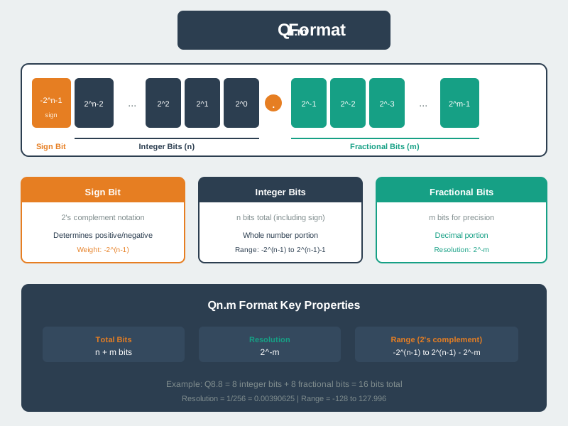
In a signed Qn.m format, n bits hold the signed integer side and m bits hold the fractional side. The stored integer maps to the real value:
\[value = \frac{stored}{2^m}\]
The smallest step is:
\[resolution = 2^{-m}\]
15.4.1 Range
The integer side must cover every expected value plus margin for abnormal inputs and intermediate states.
15.4.2 Resolution
The fractional side must be fine enough that quantization error stays within the product requirement.
15.4.3 Intermediate Width
Multiplication and accumulation usually need a wider temporary type before shifting back to the target format.
15.4.4 Saturation Policy
Define what happens when a result exceeds the format: clamp, flag, fallback, or reject the input.
15.5 Choosing A Format
Choose a format from evidence, not from a favorite convention.
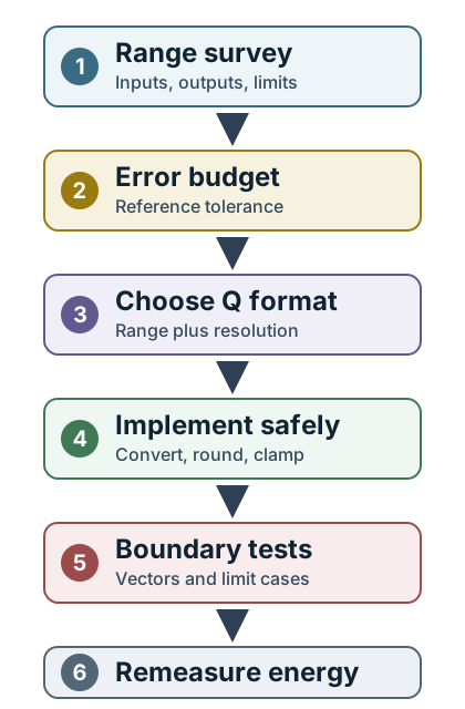
15.6 Conversion Workflow
The safest workflow is to preserve a reference implementation while you convert one numeric path at a time.
- Capture representative input ranges and edge cases.
- Define acceptable output error.
- Choose the Q-format and intermediate widths.
- Convert inputs with explicit rounding.
- Implement operations with rescaling and saturation.
- Compare fixed-point outputs against the reference.
- Remeasure full-cycle energy and timing on the target.
15.7 Core Operations
15.7.1 Conversion
To convert a real value to fixed point:
\[stored = round(value \times 2^m)\]
To convert back:
\[value = stored \times 2^{-m}\]
// Example: signed Q7.8 stored in int16_t.
#define Q_FRAC 8
#define Q_SCALE (1 << Q_FRAC)

static inline int16_t q_from_milli(int32_t milli_units) {
    // milli_units is value * 1000.
    return (int16_t)((milli_units * Q_SCALE + 500) / 1000);
}

static inline int32_t q_to_milli(int16_t q_value) {
    return ((int32_t)q_value * 1000) / Q_SCALE;
}
15.7.2 Addition
Addition is direct only when both operands use the same scale.
int16_t q_add_sat(int16_t a, int16_t b) {
    int32_t sum = (int32_t)a + (int32_t)b;
    if (sum > INT16_MAX) return INT16_MAX;
    if (sum < INT16_MIN) return INT16_MIN;
    return (int16_t)sum;
}
15.7.3 Multiplication
Multiplication doubles the fractional scale. Use a wider temporary, then shift back.
int16_t q_mul_q7_8(int16_t a, int16_t b) {
    int32_t product = (int32_t)a * (int32_t)b;  // Q14.16
    product += (1 << 7);                       // round before >> 8
    product >>= 8;                             // back to Q7.8
    if (product > INT16_MAX) return INT16_MAX;
    if (product < INT16_MIN) return INT16_MIN;
    return (int16_t)product;
}
15.7.4 Division
Division is often replaced with multiplication by a precomputed reciprocal. If division remains, widen before shifting so fractional information is not lost too early.
int16_t q_div_q7_8(int16_t numerator, int16_t denominator) {
    if (denominator == 0) {
        return numerator >= 0 ? INT16_MAX : INT16_MIN;
    }
    int32_t widened = ((int32_t)numerator << 8);
    int32_t result = widened / denominator;
    if (result > INT16_MAX) return INT16_MAX;
    if (result < INT16_MIN) return INT16_MIN;
    return (int16_t)result;
}
15.8 Overflow And Saturation
Wraparound can turn a large positive value into a negative one. For measurements, filters, and control paths, saturation plus a fault flag is often safer.
Clamp Outputs Clamp to the representable limit when the next consumer expects a bounded physical value.
Flag Faults Record that saturation happened so the system can reduce trust, retry, or enter a safe mode.
Test Boundaries Include maximum, minimum, zero, negative, and near-overflow values in regression tests.
Keep Units Visible Name variables by unit or scale so mixed-format arithmetic is visible in review.
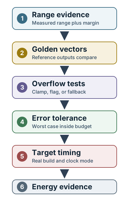
15.9 Validation Gates
Fixed-point arithmetic changes numerical behavior. Accept it only when the evidence record proves the change is safe for the product.
15.10 Review Checklist
Before accepting fixed-point firmware:
- The numeric range is measured or bounded.
- The Q-format, units, and scale are documented beside the code.
- Conversion uses explicit rounding rather than accidental truncation.
- Multiplication and accumulation use a safe intermediate width.
- Saturation or fault behavior is defined for out-of-range results.
- Golden vectors compare fixed-point output with a reference result.
- Boundary tests cover min, max, zero, negative, and near-overflow values.
- Full-cycle timing and energy are remeasured on the target build.
15.11 Check Your Understanding
15.12 Knowledge Check: Choosing A Q-Format
15.13 Knowledge Check: Multiplication
15.14 Match Fixed-Point Item To Purpose
15.15 Order The Fixed-Point Conversion Workflow
15.16 Label The Fixed-Point Design Record
15.17 On A Core Without An FPU, Every Float Is A Subroutine
Fixed-point arithmetic is usually taught as a way to save code space or gain speed, but on a battery device its biggest payoff is energy. Many low-power microcontroller cores - the Cortex-M0, M0+, and M3, for example - have no hardware floating-point unit. On those cores, every floating-point operation is executed by a software library routine that can take tens of processor cycles, while the same work in fixed-point uses ordinary integer instructions that take only a few.
Cycles are the link to energy. At a fixed clock and active current, more cycles means a longer active window, which means more energy per operation and a later return to sleep. So on an FPU-less core, choosing fixed-point over floating-point does not just run faster; it shortens how long the processor stays awake, which is where the battery is spent.
For example, compare 10000 numeric multiplies in a burst on a 16 MHz core drawing 1.5 mA while active. If software float averages 50 cycles per multiply, the burst takes 10000 x 50 / 16e6 = 31.25 ms and consumes about 1.5 mA x 0.03125 s = 0.0469 mA-s. If fixed-point averages 3 cycles, the same burst takes 1.875 ms and about 0.0028 mA-s. The operation count did not change; the active window did.
If that burst runs once per second, the difference is about 0.044 mA-s every second, or 0.044 mA of average current. Over a day that is roughly 1.06 mAh of charge, before counting any radio or sensor load.
Intuition only: without a hardware FPU, a float multiply is a function call that burns many cycles. Fixed-point turns it back into a one-cycle integer multiply, and the cycle savings become active-time and energy savings.
Why The Cost Differs
No FPU
M0, M0+, and M3 cores have no floating-point hardware, so floats run as software routines.
Soft-float cost
A software float operation can take tens of cycles; division costs even more.
Fixed-point cost
Q-format math uses integer multiply and shift, often a single-cycle multiply on the M0+.
Cycles to energy
Fewer cycles at a fixed clock means less active time and less energy per result.
Overview Knowledge Check
15.18 Cycles Become Active Time Becomes Energy
Estimate the compute energy as cycles / clock x I_active. On an FPU-less core the cycle count is where floating-point loses, and the loss multiplies across a hot loop.
Worked Example: A 1000-Tap Filter On An FPU-less Core
A filter runs 1000 multiply-accumulate operations per sample on a 16 MHz Cortex-M0+ drawing about 1.5 mA when active. Take a software single-precision multiply-accumulate at roughly 50 cycles and a Q15 fixed-point multiply-accumulate at roughly 3 cycles.
- Cycles per sample: float 1000 x 50 = 50000 cycles; fixed 1000 x 3 = 3000 cycles - about 17x fewer.
- Active time per sample: float 50000 / 16e6 = 3.125 ms; fixed 3000 / 16e6 = 0.1875 ms.
- At 100 samples per second: float keeps the core computing 312.5 ms of every second (31%); fixed keeps it computing only 18.75 ms (under 2%). Average compute current is about 0.47 mA for float versus 0.028 mA for fixed - roughly 17x, which after adding a small sleep floor still stretches battery life by more than tenfold.
The float version does not just take longer; it holds the processor out of sleep nearly a third of the time, which is what wrecks the energy budget on an FPU-less core.
That active-duty result can be turned into a battery-review number. At 1.5 mA active current, the float compute path averages about 1.5 mA x 0.3125 = 0.469 mA before other device loads. The fixed path averages about 1.5 mA x 0.01875 = 0.028 mA. Over one day of continuous sampling, compute alone is about 11.3 mAh for float versus 0.67 mAh for fixed.
Compute Energy Ledger
Practitioner Knowledge Check
15.19 The Trap Is Core-Dependent
The energy case for fixed-point depends entirely on the core. On a Cortex-M4F or M7 with a single-precision FPU, a float multiply is nearly as fast as an integer one, so fixed-point's energy edge for single-precision work largely disappears and its accuracy pitfalls may not be worth it. The decision must follow the hardware, not a habit.
But an FPU core hides a sharp trap: it accelerates only single-precision floats. A stray double-precision operation is still emulated in software, at a cost like the FPU-less case. This happens silently in C when a literal lacks the f suffix, so y = x * 0.5 promotes x to double and computes in software, whereas y = x * 0.5f stays in the hardware FPU. The same trap appears when a program calls sin instead of sinf, or assigns to a double variable. A design that expected the FPU to keep compute cheap can quietly fall back to slow software doubles, inflating active time and energy exactly as if the FPU were not there. The practitioner habit is to confirm the core, keep hot math single-precision with f-suffixed literals and single-precision library calls, and reserve fixed-point for FPU-less parts or for squeezing the last cycles.
The audit evidence is concrete. In a Cortex-M4F build, hot-path disassembly should show single-precision FPU instructions such as vmul.f32 or calls to single-precision helpers, not double-precision software routines. A map file that pulls in helpers such as __aeabi_dmul, __aeabi_dadd, or conversions between double and float is a warning that part of the numeric path escaped the hardware FPU. That evidence decides whether fixed-point is solving a real energy problem or merely adding scale-management risk.
Matching The Math To The Core
FPU-less core
Fixed-point wins clearly; every float is emulated. Prefer Q-format for hot loops.
Single-precision FPU
Hardware float is cheap; fixed-point's energy edge shrinks for single-precision work.
Accidental double
A missing f suffix or a double call falls back to slow software emulation on an SP-only FPU.
Verify, do not assume
Check the map file or disassembly to confirm hot math used the FPU, not the soft-float library.
Under-the-Hood Knowledge Check
15.20 Summary
Fixed-point arithmetic is useful when numerical requirements are clear:
- Represent real values as scaled integers.
- Select Q-format from range and precision evidence.
- Use safe intermediate widths for multiply and accumulate operations.
- Prefer explicit rounding and saturation over accidental truncation and wraparound.
- Compare against a reference with golden vectors and boundary tests.
- Remeasure timing and full-cycle energy before claiming an optimisation.
Common Pitfalls
A format with excellent resolution can still fail when a real input exceeds its integer range.
The final result may fit, but the intermediate product can overflow unless the temporary type is wide enough.
Wraparound can flip sign or hide a fault. Use saturation, flags, and boundary tests for physical values.
Fixed-point work must be remeasured across the device duty cycle. Faster math is not enough if sleep, radio, or memory behavior changes badly.
15.21 What’s Next
15.21.1 Review The Optimisation Loop
Hardware and Software Optimisation explains how to choose the right optimisation lever from evidence.
15.21.2 Tune Firmware
Software Optimization Techniques covers profiling, compiler settings, memory layout, and sleep-aware firmware.
15.21.3 Compare Hardware Paths
Hardware Optimization Strategies covers acceleration and processor selection when software changes are not enough.
15.21.4 Measure The Result
Energy Measurement and Profiling shows how to collect the before/after current trace.
15.22 Key Takeaway
Fixed-point optimization can save memory, cycles, and energy, but only when range, scaling, rounding, overflow, and accuracy are tested against the real signal and control requirements.