8 Energy Harvesting Design
Source Survey, Energy-Neutral Budgeting, Storage, and Field Verification
8.1 Start With a Cloudy Week
Energy harvesting looks easy on a sunny bench and hard during a cloudy week, a dim corridor, or a vibration pattern that stops overnight. The design question is whether the harvested trickle, storage buffer, and load policy can survive the weak periods.
Start with measured source availability, then size storage and duty cycle for energy-neutral operation instead of peak conditions.
Battery Bruno
“Every milliamp is a day of battery — budget the sleep before you budget the features.”
In this chapter, Bruno audits the harvest side too: what the trickle supplies, what the load draws, and how much storage buys the dark days.
8.2 Energy Harvesting Design
Energy harvesting can extend battery life or support energy-neutral operation, but it does not remove the need for a battery-life budget. The source is intermittent, the converter has losses, storage ages, and the IoT workload still consumes energy on its own schedule.
This chapter treats harvesting as a field design problem. Start by measuring what energy is actually available at the installation point. Then size conversion, storage, and workload policy so the device survives the worst interval, not the best afternoon.
8.3 Learning Objectives
By the end of this chapter, you will be able to:
- Survey ambient energy sources and reject sources that are too weak or intermittent.
- Build an energy-neutral ledger from measured harvest and measured load.
- Size storage for autonomy, depth-of-discharge, self-discharge, and temperature effects.
- Explain why solar, thermal, vibration, and RF harvesting have different design gates.
- Decide when MPPT or a simple converter is appropriate for a low-power node.
- Identify unrealistic indoor-solar, body-heat, and vibration assumptions.
- Specify field evidence needed before claiming perpetual operation.
- Harvesting helps only after the load is already low-power.
- Source power must be measured at the deployment point, not assumed from a catalog peak rating.
- Solar systems are usually sized by winter/dark-period energy, not summer peak output.
- Storage is part of the energy budget because it has depth-of-discharge, leakage, aging, and temperature limits.
- MPPT improves harvest only if its own quiescent current and cold-start behavior fit the source.
- “Perpetual” means energy-neutral under defined conditions, not maintenance-free forever.
Chapter path:
- First you separate source, converter, storage, and load policy so the architecture has a measurable job for each block.
- Then you compare outdoor solar, indoor light, thermoelectric, vibration, and RF sources by their real evidence gates.
- Next you close the energy-neutral ledger with the chapter’s hourly-reporting node, including 2.02 mAh per day, 83.8 mWh of dark-period storage, and a 4.2 mW winter-panel threshold.
- Finally you turn the budget into field proof: cold start, leakage, recovery after low harvest, and a policy for quiet or dark intervals.
Checkpoints recap the review decisions; the animations, calculator, and Ada audit provide the detailed arithmetic when you need it.
8.4 Harvesting Architecture
A practical harvesting system has four coupled parts: source, converter, storage, and load policy.
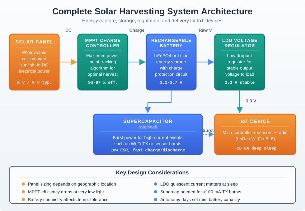
8.4.1 Source
Measure light, heat gradient, vibration, or RF availability at the installation point and through the expected low-energy interval.
8.4.2 Converter
Choose a charger, boost converter, MPPT controller, rectifier, or power-management IC that can start and operate at the measured source level.
8.4.3 Storage
Use a rechargeable battery, supercapacitor, or hybrid store sized for autonomy, burst current, leakage, temperature, and aging.
8.4.4 Load Policy
Adapt sampling, reporting, and radio behavior to the stored energy state without violating service requirements.
Converter detail matters most when the source is weak and the store is nearly empty. A harvesting power-management IC must cold-start at the measured source voltage, tolerate the source impedance, regulate or gate the load, and expose a useful power-good decision before firmware assumes energy is available.
For small stores, the charge path itself can waste a surprising amount of energy. Charging a storage capacitor in one large voltage jump loses roughly 1/2 x C x V^2 in the source and switch path. Step charging splits the rise into smaller voltage increments, so each transfer has a smaller voltage difference and less loss. A switched-capacitor or boost converter may change gain ratio, switching frequency, or load connection as the capacitor voltage rises. The review evidence should therefore include cold-start threshold, input voltage range, converter quiescent current, storage-capacitor leakage, voltage before and after a radio burst, and recovery time after a low-harvest interval.
Checkpoint: Architecture Fit
Before choosing parts, name the source condition you measured, the converter start point, the storage autonomy target, and the load state that can be reduced when energy is scarce. A design that cannot fill those four slots is still a concept sketch, not a harvesting architecture.
8.5 Source Reality Map
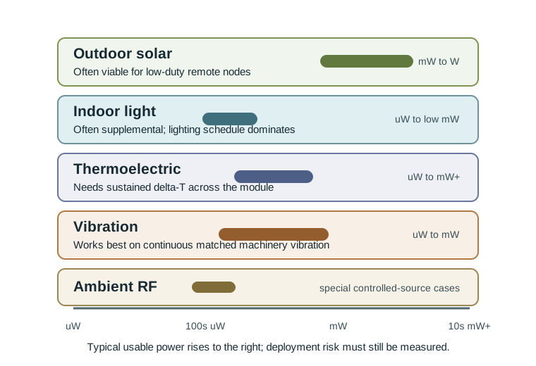
Harvesting technologies are not interchangeable. Each source has a different failure mode.
Source
Best Fit
Main Risk
Required Evidence
Outdoor solar
Remote sensors with low average load and available daylight
Winter, shading, dirt, angle, snow, dark periods
Worst-month harvest and storage autonomy record
Indoor light
Very low-power beacons near bright or persistent lighting
Lights off, low lux, spectral mismatch, small panel area
Measured lux or panel output across occupied and unoccupied periods
TEG
Sites with sustained temperature difference across the generator
Real delta-T across the module is much lower than surface-to-air temperature difference
Measured hot-side, cold-side, heatsink, and load power data
Vibration
Condition monitoring on machines with continuous, repeatable vibration
Frequency mismatch, intermittent motion, low amplitude
Acceleration spectrum and harvested power at the mounted point
RF
Special cases near a controlled RF source or reader
Ambient RF is usually too weak for normal sensor operation
Measured received power, duty cycle, and regulatory assumptions
Checkpoint: Source Evidence
Do not compare sources by name alone. Outdoor solar needs worst-month harvest and autonomy evidence, indoor light needs an occupied and unoccupied lux or panel-output record, TEGs need measured delta-T across the module, vibration needs a mounted acceleration spectrum, and RF needs received-power and duty-cycle evidence near the intended source.
8.6 Supply-Side Harvesting Examples
The demand-side answer to an energy problem is still the first answer: reduce waste, sleep aggressively, and spend computation, communication, sensing, decisions, and control only when they produce useful work. Supply-side harvesting adds a second question: is there cheap, clean, available energy at the deployment point when the node needs it?
Treat “create more energy” as a source audit, not a slogan. A hand crank or emergency radio may produce tens of watts per kilogram while a person is turning it; a shake flashlight proves magnetic induction but not continuous service; a shower-head turbine may have only milliwatts while water is flowing; a roadway harvester may claim kilowatts per car but has civil-work, traffic, and maintenance costs. The common review move is to convert each example into a measured source profile, then compare it with the load and storage ledger.
| Source idea | Example from the slide deck | Design lesson |
|---|---|---|
| Magnetic generator | Wind turbine, hand crank, shake flashlight | Motion plus a magnetic field can induce useful current, but the source exists only when the motion exists. |
| Mechanical pressure or motion | Water pressure around 1.5 mW / 60 psi, shoe-mounted cranks, speed-bump harvesters claiming 5-50 kW / car |
Power density can look impressive at the source but may not match a small node’s schedule, maintenance budget, or installation cost. |
| Thermoelectric | Self-powered watch around 22 uW, exhaust or engine waste-heat recovery around kilowatt scale |
Temperature difference is the source; the design must prove real delta-T across the generator and a heat path that lasts. |
| Atmospheric temperature or pressure | Wireless sensor nodes powered from ambient temperature changes | Slow ambient changes can support rare reporting, but they require long accounting windows and storage-aware communication. |
| Piezoelectric stress or strain | PZT shoe inserts and stress/strain harvest circuits | Repeatable vibration or strain can help tiny loads, while random footsteps are weak unless the application can tolerate sparse harvest. |
| RF scavenging | Passive UHF RFID-style tags and object-interaction systems near a reader | Reader-provided RF can wake a tag and support backscatter or a short transaction; ambient RF is not a general battery replacement. |
| RF-powered sensing | WISP-style sensor or camera nodes, such as 176 x 144 images at about 0.1 fps |
Wireless power only closes when source field, receiver orientation, duty cycle, payload size, and user expectation are designed as one envelope. |
This is why the source map above is paired with the field record below. The holy grail is not simply harvesting more energy than the node needs on a good moment; it is closing the ledger across the worst interval without hiding availability, conversion, storage, or maintenance costs.
8.7 Energy-Neutral Ledger
The design is energy-neutral only if the storage state recovers over the chosen accounting window.
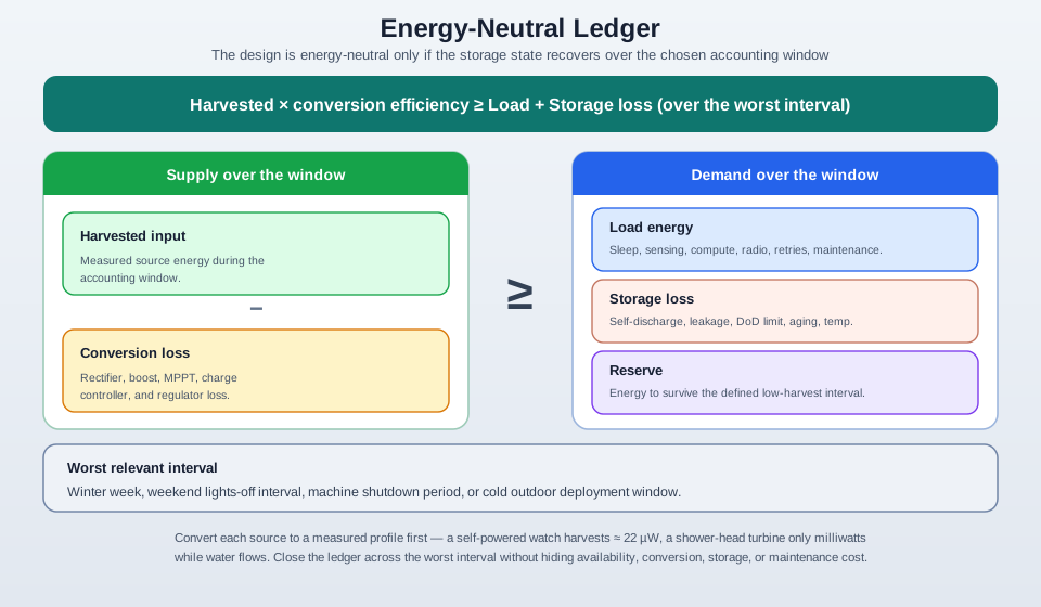
Use this accounting form:
- Harvested input: measured source energy during the accounting window.
- Conversion loss: rectifier, boost, MPPT, charge controller, and regulator loss.
- Load energy: sleep, sensing, compute, radio, retries, and maintenance states.
- Storage loss: self-discharge, leakage, depth-of-discharge limit, aging, and temperature derating.
- Reserve: the energy needed to survive the defined low-harvest interval.
Energy-neutral operation means:
\[E_{\text{harvested}} \times \eta_{\text{conversion}} \ge E_{\text{load}} + E_{\text{storage loss}}\]
That inequality must hold over the worst relevant interval, such as winter week, weekend lights-off interval, machine shutdown period, or cold outdoor deployment window.

8.7.1 Phoebe’s Why
Harvesting starts with a transducer, but the node survives only if the store refills over the review window. A solar cell turns photon flux into current and has one voltage where current times voltage is largest. A thermoelectric generator turns temperature difference into voltage. A piezo element turns strain into charge. Those sources are different at the device level, but the system test is the same: harvested energy after conversion must cover load energy plus the buffer needed for dark, cold, shaded, or still intervals.
8.7.2 The Derivation
A photovoltaic cell is a light-driven diode. Photon flux creates photocurrent \(I_{ph}\), while the junction still follows the diode law:
\[I = I_{ph} - I_0\left(e^{qV/(n kT)} - 1\right)\]
Electrical output power is
\[P(V) = V I(V)\]
The maximum-power point is where
\[\frac{dP}{dV} = I + V\frac{dI}{dV} = 0\]
so an MPPT controller keeps moving the operating voltage until the extra voltage no longer pays for the current it gives up.
A thermoelectric generator starts from the Seebeck effect:
\[V_{oc} = S\Delta T\]
With internal resistance \(R_i\) and load \(R_L\),
\[I = \frac{S\Delta T}{R_i + R_L}\]
Maximum load power occurs at \(R_L = R_i\):
\[P_{max} = \frac{(S\Delta T)^2}{4R_i}\]
A piezo element starts from charge generated by force:
\[Q = dF\]
If its capacitance is \(C_p\), the open-circuit voltage and stored event energy are
\[V = \frac{Q}{C_p}\]
\[E = \frac{1}{2}C_pV^2 = \frac{Q^2}{2C_p}\]
All three sources then enter the same ledger:
\[E_h\eta_c \ge E_L + E_{loss}\]
8.7.3 Worked Numbers: This Chapter’s Solar Ledger
- Hourly node load: sleep uses \(0.018\,\text{mA}\times24\,\text{h}=0.432\) mAh/day; sensing uses \(6\,\text{mA}\times3\,\text{s}\times24/3600=0.120\) mAh/day; radio uses \(110\,\text{mA}\times2\,\text{s}\times24/3600=1.47\) mAh/day. Total \(=2.02\) mAh/day.
- Daily energy: \(2.02\,\text{mAh}\times3.3\,\text{V}=6.67\) mWh/day, which is the chapter’s
6.7 mWh/dayrounded for the review ledger. - Dark-period storage: using the chapter’s rounded \(6.70\) mWh/day, seven low-harvest days need \(6.70\times7=46.9\) mWh of load energy. With \(80\%\) usable depth and a \(30\%\) reserve, required storage is \(46.9/(0.8\times0.7)=83.8\) mWh.
- Winter panel threshold: if only two useful harvest hours are available and charger efficiency is \(80\%\), the panel must supply \(6.70/(2\times0.8)=4.19\) mW during those hours, reported in the chapter as about \(4.2\) mW.
- Outdoor versus indoor scale: one square centimeter of outdoor solar at \(15\) mW/cm2 for \(2\) peak-sun-hours with a \(0.7\) derating gives \(15\times2\times0.7=21.0\) mWh/day, enough for a \(0.5\) mW load that needs \(0.5\times24=12.0\) mWh/day. Indoors, \(10\) uW/cm2 for \(10\) lit hours with the same derating gives \(0.010\times10\times0.7=0.0700\) mWh/day per cm2, so that same load needs \(12.0/0.0700=171\) cm2 before storage losses.
8.8 Communication Under Random Energy Dynamics
A conventional battery-powered radio often starts from a fixed transmit-power budget. A harvesting transmitter has a different problem: energy arrives over time, may be random, and is often known only when the device has already harvested it. The communication design must therefore respect both the channel and the storage state.
For a simple slot model, let E_t be the harvested energy arrival, B_t the stored energy available before transmission, and X_t the transmitted signal in that slot. The transmitter can spend only what is in the store:
\[|X_t|^2 \le B_t\]
After the slot, the next storage state is bounded by the storage size:
\[B_{t+1} = \min(B_t - |X_t|^2 + E_{t+1}, B_{\max})\]
This is the technical version of the ledger above. Source variability changes when the node can transmit, not only how much energy it uses per day. If a gateway or receiver does not know the harvest process, the protocol should tolerate deferred reports, shorter payloads, local buffering, or explicit low-energy status instead of treating silence as only a link failure.
In the ideal limit where storage is effectively unlimited, the long-run capacity of an additive white Gaussian noise channel can be treated like the classical Shannon channel with average transmit power equal to the average harvesting rate:
\[C = W \log_2\left(1 + \frac{\mathbb{E}[E_t]}{N_0 W}\right)\]
Finite storage changes the question. If B_{\max} is larger than the largest likely energy arrival, the store behaves close to the average-power case above. If B_{\max} clips arrivals, the useful transmit budget is closer to the average of min(E_t, B_{\max}) because excess harvest is spilled instead of saved. Correlated arrivals matter as much as the mean: a long low-harvest coherence interval can drain the store even when the long-run average looks acceptable, while clustered high-harvest intervals may be wasted if the store is already full.
The engineering lesson is narrow but useful: average harvested energy determines the theoretical link budget, while finite storage, cold-start behavior, and causal knowledge of E_t determine the field schedule. Use ordinary communication and coding techniques only after the measured harvest average closes; then add a storage-aware policy for the bad intervals. A good review states which regime the node is in, whether increasing B_{\max} is still useful, and whether the better fix is a larger store, a lower payload rate, or a different transmit-power policy.
Remotely powered communication adds one more coordination boundary. A charger may transfer energy at a fixed rate, observe only past channel outputs, observe intended transmitter inputs, or share richer side information about the transmitter’s battery state. More side information can let the charger time energy transfer closer to the moments when the transmitter needs it, but it is not free: the design must account for observation cost, control latency, regulatory power limits, and what the receiver should infer from silence. Record whether the transmitter adapts coding or modulation to instantaneous battery level and whether the gateway can distinguish low-energy silence from an ordinary link failure.
8.9 Worked Example: Outdoor Solar Sensor
Scenario: A low-power environmental node reports once per hour. A field measurement shows:
- Sleep baseline: 18 uA for almost the full hour.
- Sensing and compute: 6 mA for 3 seconds each hour.
- Radio transaction: 110 mA for 2 seconds each hour.
- System voltage: 3.3 V.
Daily load estimate:
- Sleep:
0.018 mA x 24 h = 0.432 mAh/day. - Sensing:
6 mA x 3 s x 24 / 3600 = 0.120 mAh/day. - Radio:
110 mA x 2 s x 24 / 3600 = 1.467 mAh/day. - Total: about
2.02 mAh/day. - Energy:
2.02 mAh x 3.3 V = 6.7 mWh/day.
Storage for 7 low-harvest days:
- Load over 7 days:
6.7 x 7 = 46.9 mWh. - With 80% usable depth and 30% reserve:
46.9 / 0.8 / 0.7 = 83.8 mWh. - At 3.2 V nominal storage, this is about
26 mAh; choose a larger standard cell after temperature and aging review.
Panel sizing:
- If the worst useful winter harvest window is 2 hours per day, and charger efficiency is 80%, the panel must deliver at least
6.7 / (2 x 0.8) = 4.2 mWaverage during those useful hours. - Add site margin for angle, dirt, shading, seasonal uncertainty, and battery recharge after a dark period.
Design decision: The first sizing result is small because the node is already low-power. The review is not complete until the team measures the actual panel at the site, verifies charger cold start, and tests recovery after a multi-day dark interval.
Bruno’s Power Budget
- Draw: 18 uA sleep, 6 mA sense, 110 mA radio — 2.02 mAh (6.7 mWh) per day.
- Sleep: asleep almost the full hour between hourly reports — the 2-second radio burst dominates.
- Life: seven dark days need 83.8 mWh stored, plus at least 4.2 mW of winter panel.
Checkpoint: Energy-Neutral Math
Recompute the ledger before accepting the result: 0.432 + 0.120 + 1.467 = 2.019 mAh/day, about 2.02 mAh/day; 2.02 x 3.3 = 6.7 mWh/day; 6.7 x 7 / 0.8 / 0.7 = 83.8 mWh; and 6.7 / (2 x 0.8) = 4.2 mW. The arithmetic is small, but each line must be tied to measured deployment assumptions.
8.10 MPPT and Converter Gates
MPPT is not automatically better for every small node. It helps when the source has a moving maximum-power point and the controller overhead is small compared with harvested power.
Use MPPT when The source power is large enough to pay for controller overhead, the operating point changes with light or temperature, and the storage charger can cold-start at the measured source voltage.
Use simpler conversion when The source is extremely weak, the load is tiny, the operating point is stable, or the MPPT quiescent current would consume too much of the harvest.
Always verify Cold start, quiescent current, leakage, input voltage range, storage protection, and efficiency at the actual micro-watt or milli-watt load level.
Avoid component tables that imply a part is universally correct. The right converter depends on source voltage, source impedance, cold-start requirement, storage chemistry, leakage budget, and load bursts.
8.11 Storage Design
Storage must handle two different jobs: long gaps between harvest events and short bursts from the load.
8.11.1 Rechargeable Battery
Good for multi-hour or multi-day autonomy. Check charge temperature limits, depth of discharge, cycle life, protection, and aging.
8.11.2 Supercapacitor
Good for high-cycle buffering and short bursts. Check self-discharge, usable voltage range, regulator dropout, and leakage.
8.11.3 Hybrid Store
Useful when a battery supplies long autonomy and a capacitor handles radio bursts or sensor pulses.
For a burst buffer, the usable capacitor energy is:
\[E = \frac{1}{2} C \left(V_{\text{high}}^2 - V_{\text{low}}^2\right)\]
Use that equation only after checking equivalent series resistance, leakage, and the minimum voltage accepted by the regulator and load.
8.12 Indoor and Non-Solar Reality Checks
Harvesting proposals often fail because the source was described qualitatively instead of measured.
Indoor light can support very low-power devices, especially with cells designed for indoor spectra, but many IoT nodes consume more than a small indoor panel can provide. Measure panel output under the actual lighting schedule, including nights, weekends, shades, occupancy sensors, and fixture changes.
A hot pipe or warm enclosure is not enough. Thermoelectric output depends on the temperature difference across the module after thermal contact resistance and heatsink limits are included.
Piezoelectric harvesters are useful on some rotating machinery and other repeatable vibration sources. They are usually weak for random structural motion, footsteps, and intermittent movement unless the load is extremely small.
Ambient RF is rarely a general-purpose power source for normal sensing nodes. Treat RF harvesting as viable only near a controlled transmitter, reader, or intentionally designed energy source.
An RF harvesting record should name the coupling mode, antenna or coil geometry, matching network, rectifier, storage capacitor, distance, alignment, regulatory limit, and measured harvested voltage under load. A near-field reader or phone tap can support a short wake/store/sleep transaction; that does not prove a far-field ambient deployment can run the same node continuously.
8.13 Field Verification Record
Before claiming energy-neutral operation, record evidence that can be retested.
Record Field
Required Detail
Why It Matters
Pass/Fail Question
Source
Measured output by time, season, orientation, mounting point, or operating condition
Catalog ratings do not represent the installation
Was worst-case source availability measured or bounded?
Load
Whole-device state current, timing, retry behavior, and maintenance states
Harvesting cannot rescue an unmeasured load
Does the load ledger use measured values?
Storage
Capacity, usable depth, leakage, temperature, aging, and burst-current evidence
Storage determines survival through low-harvest intervals
Can the node survive the defined autonomy period?
Recovery
Recharge time after dark, cold, shaded, quiet, or low-source intervals
Energy-neutral systems must recover, not only survive
Does the storage state recover before the next low-harvest interval?
Checkpoint: Field Proof
A passing field record answers four questions in order: was the source measured under weak conditions, was the whole-device load measured across sleep and bursts, can storage survive the defined low-harvest interval, and does the store recover before the next weak interval arrives?
8.14 Common Pitfalls
Peak panel, TEG, or harvester ratings are not the same as deployed daily energy. Use measured site output and worst-case intervals.
Rectifiers, boost converters, MPPT controllers, regulators, battery charging, self-discharge, and protection circuits all consume part of the harvest.
Energy-neutral operation with a finite battery or capacitor must survive low-harvest periods and then recover. Otherwise the node slowly drains over repeated bad intervals.
A harvesting node needs a policy for low-energy conditions: reduce sample rate, defer reporting, buffer locally, or enter a safe mode while preserving required service.
8.15 Knowledge Check
8.16 Quiz: Energy-Neutral Budget
8.17 Matching Quiz: Source to Design Gate
8.18 Ordering Quiz: Harvesting Design Review
8.19 Label the Diagram: Harvesting Energy Path
8.21 What’s Next
8.21.1 Use Interactive Tools
Use calculators after the source and load ledgers are measured.
8.21.2 Reduce Load First
Reduce the load before sizing a harvesting system.
8.21.3 Compare Field Evidence
Compare harvesting claims with measured field evidence patterns.
8.22 Harvest Is A Trickle, So Budget Averages And Store The Rest
Energy harvesting replaces or supplements a battery by pulling power from the environment. The catch is scale: ambient sources deliver a trickle compared with a battery's reserve, and that trickle is intermittent. Designing a harvesting node is therefore an averages-and-storage problem, not a peak-power one. You compare the average power you can harvest against the average power the device consumes, and you add storage to ride through the gaps when the source is absent.
The sources differ by orders of magnitude, and knowing the rough numbers keeps a design honest. Representative electrical output densities are about 15 mW per square centimeter for outdoor solar, only about 10 microwatts per square centimeter for indoor solar, tens of microwatts per square centimeter for a body-heat thermoelectric generator, around 100 microwatts per cubic centimeter for machine-vibration piezo, and well under 1 microwatt per square centimeter for ambient radio-frequency energy.
A quick budget exposes the difference. A 0.5 mW sensor needs 0.5 x 24 = 12 mWh/day. One square centimeter of outdoor solar with 2 peak-sun-hours and a 0.7 derating can produce about 15 mW x 2 h x 0.7 = 21 mWh/day, so the daily energy balance closes. Indoors, the same square centimeter at 10 uW for 10 lit hours and 0.7 derating produces only 0.07 mWh/day; the same load would need about 12 / 0.07 = 171 cm2 before storage losses. The source choice changes the physical design, not just the BOM line.
Intuition only: harvesting works when average harvested power, after weather and conversion losses, is at least the device's average load - and when storage can carry the load through the longest dark or still period.
Source Reality
Solar
Best density outdoors (about 15 mW/cm2) but roughly a thousand times weaker indoors. Highly time-varying.
Thermoelectric
Tens of microwatts per square centimeter from a small temperature difference; more with a large industrial delta-T.
Vibration / piezo
Around 100 microwatts per cubic centimeter from machinery; far less from gentle human motion.
Ambient RF
Under 1 microwatt per square centimeter from stray transmitters - the weakest common source.
Overview Knowledge Check
8.23 Size For Energy-Neutral, Not Peak
Convert the intermittent source into a daily energy using peak-sun-hours (PSH), the equivalent hours per day at full rating. Then require panel_daily_energy x derating >= load_daily_energy and size storage for the longest expected gap.
Worked Example: Outdoor Solar Sensor
The device averages 0.2 mA at 3.3 V, which is 0.66 mW, or 15.8 mWh per day. Use a conservative 2 peak-sun-hours per day for reliability in poor weather and a system derating of 0.7 for conversion, dirt, and angle losses.
- Panel size: required panel peak power = 15.8 mWh / (2 h x 0.7) = 11.3 mW. At 15 mW/cm2 outdoors, that is only about 0.75 cm2 of cell - a postage stamp comfortably powers this load.
- Storage for autonomy: to survive 3 days with no harvest, store 15.8 mWh x 3 = 47.5 mWh. At 3.7 V that is about 12.8 mAh, met by a small 20-50 mAh lithium cell.
- Result: the outdoor design is generous; the panel is tiny and a small cell provides multi-day ride-through.
Notice the two independent sizes: the panel is sized by the daily energy balance, and the storage is sized by the worst-case gap. Getting one right does not excuse the other.
Then add engineering margin before calling it viable. If the site spends one winter week at only 1 peak-sun-hour, the same panel harvests 11.3 mW x 1 h x 0.7 = 7.9 mWh/day, half the load. A controller can respond by stretching the reporting interval, disabling a high-current sensor, or declaring a maintenance fault before the buffer reaches brownout. The harvesting budget therefore needs both a nominal sizing line and a degraded-mode policy line.
Bruno’s Power Budget
- Draw: 0.2 mA at 3.3 V is 0.66 mW — 15.8 mWh per day.
- Sleep: a one-peak-sun-hour winter week harvests 7.9 mWh/day, half the load — stretch reporting before brownout.
- Life: three no-harvest days need 47.5 mWh — about 12.8 mAh at 3.7 V, a small 20-50 mAh cell.
Harvesting Sizing Ledger
Practitioner Knowledge Check
8.24 Indoor Is A Thousand Times Weaker, And Peak Is Not Average
The most common harvesting mistake is moving an outdoor-proven solar node indoors. Outdoor cell output is around 15 mW/cm2; typical office lighting yields only about 10 uW/cm2 - roughly a thousandfold drop. Take the same 15.8 mWh/day load. Indoors, with light available perhaps 10 hours a day, a square centimeter gathers about 10 uW x 10 h = 0.1 mWh per day. Meeting the load after derating needs about 22.6 mWh/day, which demands roughly 226 cm2 of indoor cell - a sheet the size of a page - versus under 1 cm2 outdoors. The panel that trivially powers the outdoor node cannot power the indoor one.
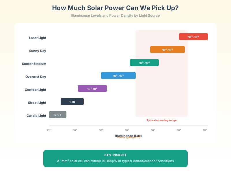
The second trap is confusing peak power with average power. A cell rated 15 mW/cm2 delivers that only in full sun. Rating a node on the peak overstates the daily harvest by the ratio of a full day to the actual peak-sun-hours, and the shortfall is worst in the season you can least afford it. Storage type follows from the gap length: for a few hours of ride-through a supercapacitor works and tolerates endless cycles, but for days of autonomy the energy needed forces a battery, because a supercapacitor large enough would be impractical.
Buffer math uses usable energy, not nameplate energy. A 50 mAh lithium buffer at 3.7 V stores about 50 x 3.7 = 185 mWh, but an 80% depth-of-discharge limit leaves 148 mWh. That covers the 15.8 mWh/day example for about 148 / 15.8 = 9.4 days before converter quiescent current, cold derating, and aging. A 10 uA always-on charger path at 3.7 V consumes another 0.010 mA x 3.7 V x 24 h = 0.89 mWh/day, which is small outdoors but material indoors.
Bruno’s Power Budget
- Draw: 15.8 mWh/day of load plus 0.89 mWh/day from a 10 uA always-on charger path.
- Sleep: hours of gap suit a supercapacitor; days of autonomy force a battery.
- Life: a 50 mAh cell holds 185 mWh, 148 usable at 80 percent depth — about 9.4 days of ride-through.
Reality Checks Before Committing
Indoor gap
Indoor light is about a thousand times weaker than outdoor. Re-measure at the real install location, not in sunlight.
Peak-sun-hours
Size on equivalent full-rating hours in the worst season, not on the panel's peak plate rating.
Storage horizon
Hours of autonomy favor a supercapacitor; days of autonomy require a battery. Match the buffer to the gap.
Cold-charge limit
If the buffer is Li-ion, a cold outdoor site cannot charge it below 0 C without damage; gate charging by temperature.
Under-the-Hood Knowledge Check
8.25 Summary
This chapter introduces energy harvesting sources such as solar, vibration, thermal, and RF. It connects harvested power, storage, load profiles, energy-neutral operation, and reliability during low-input periods.
8.26 Key Takeaway
Energy harvesting works only when the long-term energy balance closes. Size storage for gaps, measure realistic source availability, and design graceful behavior for periods when harvested power is below demand.