18  Lab: Energy Measurement

Measuring Sleep, Wake, Radio, and Duty-Cycle Behavior on an IoT Node

18.1 Start With the Meter in Series

The lab begins when the meter is in the current path and the firmware change is visible on the trace. A sleep setting, wake source, or duty-cycle policy is not complete until the measured device behaves as expected.

Use the exercises as a loop: predict the state current, flash the firmware, capture the trace, explain mismatches, and keep the evidence with the design note.

In 60 Seconds

This lab turns energy-aware design into evidence. You will define a workload, measure whole-device current in each state, implement a timer-based sleep loop, test wake-source behavior, calculate average current, and record whether the measured node meets its battery-life target.

Phoebe’s Field Notes: The Shunt You Choose Can Falsify the Sleep Current You’re Measuring

Phoebe’s Why

This lab’s own safety warning – “start with a current range that can tolerate the board’s startup and radio current, then move to a lower range for sleep-current measurement” – is really a circuit-physics statement in disguise. A shunt-based current measurement works by inserting a small resistor in series and reading the voltage it drops, but that same insertion adds a real resistor into the device’s own supply path. Size it to comfortably resolve microamp sleep current and it will drop volts at the radio’s peak current, dragging the whole board’s rail down mid-measurement. Size it to survive the radio peak safely and its sleep-current voltage drop can fall below what the meter can resolve. The four states in this chapter’s own Baseline State Ledger span several orders of magnitude of current for exactly this reason.

The Derivation

The shunt’s own voltage drop – the “burden voltage” it inserts into the measured circuit – follows directly from Ohm’s law:

\[V_{burden} = I\,R_{shunt}\]

The measured average current for one complete cycle is the charge-weighted sum this chapter’s own Baseline State Ledger instructs you to build:

\[I_{avg} = \frac{\sum_i I_i\,t_i}{\sum_i t_i} = \frac{Q_{total}}{T_{total}}\]

A single fixed shunt must satisfy both ends of the current range at once, which is why the dynamic range between the highest and lowest state current is the number that decides whether one shunt value can serve the whole trace:

\[\text{dynamic range (dB)} = 20\log_{10}\!\left(\frac{I_{max}}{I_{min}}\right)\]

Worked Numbers: A Catalog-Typical ESP32-Class Cycle

The chapter’s own firmware fixes \(\mathrm{SLEEP\_SECONDS}=900\) and a \(250\) ms sensor warm-up (delay(250)); take catalog-typical state currents for the rest: boot \(130\) mA for \(100\) ms, sensor warm-up \(5\) mA for \(250\) ms, a radio burst \(120\) mA for \(50\) ms, and deep sleep \(10\ \mu\)A for the remaining \(900\) s.

• \(Q_{total} = (0.130\times0.100)+(0.005\times0.250)+(0.120\times0.050)+(10\times10^{-6}\times900) = 0.02925\) A\(\cdot\)s over \(T_{total}=900.4\) s, giving \(I_{avg}=32.5\ \mu\)A – this is the number the Baseline State Ledger’s “sum of all state contributions” instruction is asking you to compute.
• Dynamic range: \(I_{max}/I_{min} = 0.120/0.00001 = 12{,}000\times\), or \(81.6\) dB – almost five decades on one trace.
• A \(10\ \Omega\) shunt (sized to make sleep current visible: \(10\ \mu\mathrm{A}\times10\ \Omega=100\ \mu\)V) drops \(0.120\,\mathrm{A}\times10\,\Omega=1.20\) V at the radio peak – over a third of a 3.3 V rail, easily enough to brown out the very radio session being measured.
• A \(1\ \Omega\) shunt keeps the radio-peak burden to a safe \(120\) mV, but the sleep-current signal falls to \(10\ \mu\mathrm{A}\times1\,\Omega=10\ \mu\)V – likely below many meters’ noise floor. This is the exact physics behind this lab’s own instruction to change current range between states rather than trust one fixed setting for the whole cycle.

18.2 Hands-On Energy Measurement Lab

This chapter is a lab, not a product recipe. Use the board, radio, and sensor platform available in your course or project. The examples use ESP32-style sleep APIs because they are familiar in IoT labs, but the method applies to any low-power microcontroller.

The goal is to produce a defensible energy record: measured current, measured timing, workload assumptions, calculated average current, and a clear pass/fail decision against the target lifetime.

18.3 Learning Objectives

By the end of this lab, you will be able to:

• Set up a safe whole-device current measurement path.
• Measure sleep, sensor warm-up, active compute, radio, and wake-transition states.
• Implement a timer-based sleep loop and preserve state across wake cycles.
• Compare timer wake, GPIO wake, and adaptive duty-cycle policies.
• Calculate average current from a measured cycle trace.
• Explain why simulator or datasheet values are not enough for battery-life approval.
• Write an evidence record that another engineer can reproduce.

Minimum Viable Understanding

• A lab trace must include the whole device, not only the microcontroller.
• Sleep-mode firmware is incomplete until sensors, regulators, pull-ups, LEDs, and radios are also controlled.
• Timer wake is predictable; GPIO wake can save energy only if false triggers are controlled.
• Adaptive sampling saves energy only when the high-rate mode is rare and bounded.
• Battery-life estimates must be based on measured current and measured time.
• A simulator can validate logic flow, but hardware measurement validates energy.

18.4 Lab Workflow

Follow the lab in six passes. Do not jump straight to the final battery-life calculation.

Figure 18.1: Hands-on energy lab workflow showing requirement, measurement setup, baseline trace, sleep firmware, policy experiment, and evidence record.

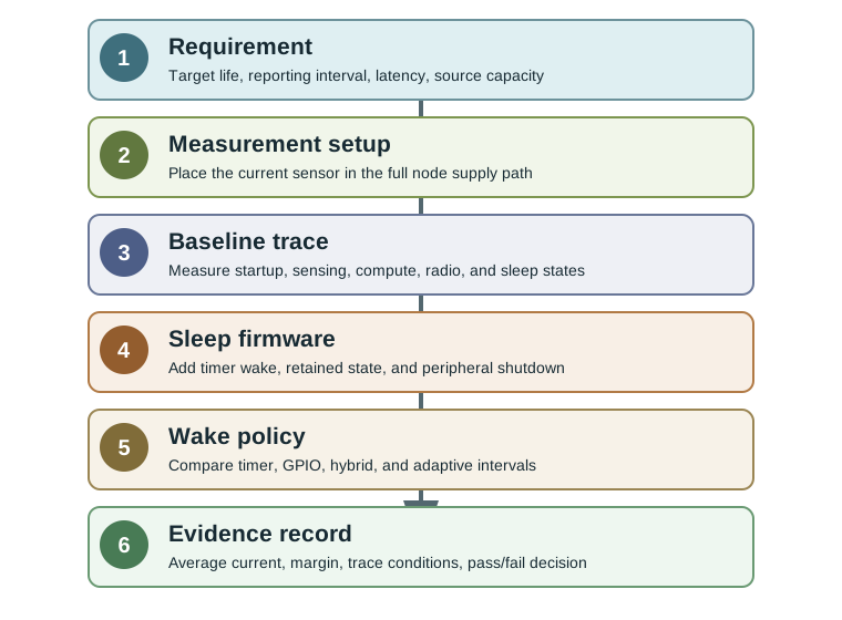
18.4.1 1. Requirement

Write the target service: sample interval, reporting interval, latency, lifetime, source capacity, and accepted data loss.

18.4.2 2. Setup

Insert a current meter, current probe, shunt amplifier, or power profiler so it measures the full node supply path.

18.4.3 3. Baseline

Measure the current and duration of each normal state before changing firmware.

18.4.4 4. Sleep Loop

Add timer sleep, state retention, and peripheral shutdown. Measure again.

18.4.5 5. Wake Policy

Compare fixed timer wake, GPIO wake, and adaptive interval logic against the workload.

18.4.6 6. Evidence

Calculate average current, check margin, and record the trace conditions.

18.5 Equipment and Safety

Use equivalent tools if your lab kit differs.

• IoT development board with a sleep mode, such as an ESP32-class board or a low-power Cortex-M board.
• Sensor or load that can be enabled and disabled by firmware.
• Current-measurement tool: power profiler, current probe, inline ammeter, shunt resistor plus differential measurement, or source-measure unit.
• Stable supply or battery emulator set to the deployment voltage.
• Optional radio or network connection if the lab includes a transmit state.
• Notebook or spreadsheet for state current, state duration, and calculation records.

Measurement Safety

Do not place an ammeter directly across a power supply. It must be in series with the load. Start with a current range that can tolerate the board’s startup and radio current, then move to a lower range for sleep-current measurement.

18.6 Measurement Setup

The current sensor belongs in the supply path that powers the whole node. If USB remains connected, the USB interface and debugger may hide the real sleep current.

Figure 18.2: Energy lab measurement setup showing supply, current sensor, device under test, firmware trace, and state ledger.

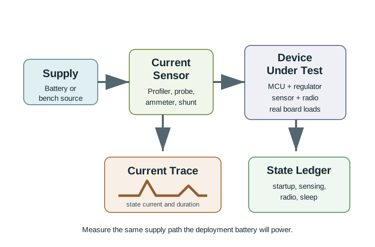
Before taking measurements:

1. Power the board from the same supply rail you intend to measure.
2. Disconnect or account for USB debug power.
3. Confirm the measurement tool can capture both short radio peaks and low sleep current.
4. Disable automatic LEDs, debug UARTs, and peripherals only after recording the baseline.
5. Record firmware version, supply voltage, sensor configuration, radio configuration, and ambient condition.

18.7 Baseline State Ledger

Measure at least one complete cycle and separate it into states.

State

What to Measure

Common Surprise

Evidence to Record

Startup

Boot current, boot duration, reset reason

Startup can last longer than the useful sensing work

Trace segment, firmware version, supply voltage

Sensing

Sensor warm-up, conversion, and bus activity

Warm-up time can dominate low-rate sensors

Sensor enable pin state and valid-reading rule

Radio

Attach, transmit, receive, acknowledgement, retries

Poor coverage can multiply radio time

Payload size, retry policy, signal condition

Sleep

Whole-board current after settling

Regulators, pull-ups, sensors, and debug chips keep drawing current

Settling delay, final current, enabled wake sources

Use the same units across the ledger. For each state, multiply the state current by the fraction of the cycle spent in that state. The sum of all state contributions is the measured average current for the cycle.

18.8 Exercise 1: Baseline Trace

Task: Measure the unoptimized node through one complete sense-and-report cycle.

Record:

• Supply voltage.
• Startup duration and peak current.
• Sensor warm-up current and duration.
• Active compute current and duration.
• Radio or logging current and duration.
• Idle or sleep current after the active work finishes.
• Cycle period used for the calculation.

Acceptance Check

Your baseline is acceptable only if another person can reproduce the trace from your notes. “It used about 20 mA” is not enough. Record the firmware, supply, measurement range, workload, and where each state starts and ends.

18.9 Exercise 2: Timer Sleep Firmware

Timer sleep is the simplest low-power loop: wake, measure, decide, report, prepare peripherals, sleep.

Figure 18.3: Sleep-mode firmware loop showing wake reason, retained state, measurement, reporting, peripheral shutdown, and timer sleep.

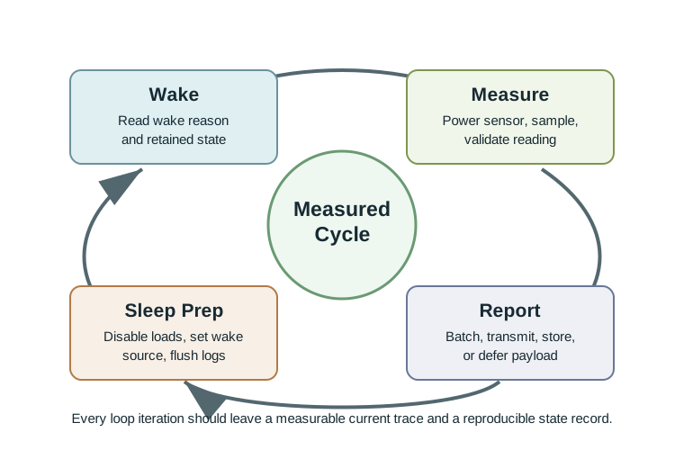
The following ESP32-style snippet shows the pattern. Adapt the pin names, radio shutdown, and sensor controls to your board.

#include <Arduino.h>
#include <esp_sleep.h>

constexpr uint64_t SLEEP_SECONDS = 900;
constexpr int SENSOR_ENABLE_PIN = 12;
constexpr int STATUS_LED_PIN = 2;

RTC_DATA_ATTR uint32_t wakeCount = 0;

void preparePeripheralsForSleep() {
  digitalWrite(STATUS_LED_PIN, LOW);
  pinMode(STATUS_LED_PIN, INPUT);

  digitalWrite(SENSOR_ENABLE_PIN, LOW);
  pinMode(SENSOR_ENABLE_PIN, OUTPUT);

  // Add board-specific radio shutdown here.
  // Example: disconnect Wi-Fi/BLE or put the modem into its lowest-power state.
}

void setup() {
  Serial.begin(115200);
  delay(100);

  esp_sleep_wakeup_cause_t cause = esp_sleep_get_wakeup_cause();
  if (cause == ESP_SLEEP_WAKEUP_UNDEFINED) {
    wakeCount = 0;
  }
  wakeCount++;

  pinMode(STATUS_LED_PIN, OUTPUT);
  pinMode(SENSOR_ENABLE_PIN, OUTPUT);

  digitalWrite(SENSOR_ENABLE_PIN, HIGH);
  delay(250);
  int reading = analogRead(A0);

  Serial.printf("Wake %lu, cause %d, reading %d\n",
                (unsigned long)wakeCount,
                static_cast<int>(cause),
                reading);

  preparePeripheralsForSleep();
  Serial.flush();

  esp_sleep_enable_timer_wakeup(SLEEP_SECONDS * 1000000ULL);
  esp_deep_sleep_start();
}

void loop() {
  // Execution restarts in setup() after deep sleep.
}

Measure the trace again after adding the sleep loop. The important question is not “did the API compile?” The important question is “did the measured whole-device sleep current fall enough to meet the design contract?”

18.10 Exercise 3: Wake-Source Policy

Compare at least two wake policies.

18.10.1 Fixed Timer Wake

The node wakes on a schedule. It is predictable and easy to budget, but it may waste energy when nothing changes.

18.10.2 GPIO Event Wake

The node wakes on an external signal. It can save energy for rare events, but false triggers can destroy the budget.

18.10.3 Hybrid Wake

The node wakes on both a slow timer and an event signal. This supports periodic health checks and urgent events.

For each policy, record:

• Wake source and configuration.
• Number of wakeups during the test window.
• Average active time per wake.
• False trigger count or missed-event count.
• Resulting average current.

Review Trap: GPIO Wake Without False-Trigger Testing

GPIO wake is energy efficient only when event triggers are rare and meaningful. A noisy motion sensor, floating input, or unfiltered switch can wake the node hundreds of times per day.

18.11 Exercise 4: Adaptive Duty Cycling

Adaptive duty cycling changes the next sleep interval based on measured conditions. The policy must be bounded, measurable, and reversible.

Run it: Before you script the sequence below, model the same policy in the context-aware energy optimizer below. Set how the node reacts to change – short intervals when readings move, longer intervals when they stay quiet – and watch the average current and responsiveness trade off against each other. Use it to find a bounded interval range that still catches events, then compare its predicted average current with the fixed-interval baseline when you record whether adaptive mode actually saves energy.

uint32_t chooseNextSleepSeconds(float currentValue, float previousValue, uint8_t quietCount) {
  float delta = fabs(currentValue - previousValue);

  if (delta > 2.0f) {
    return 60;        // Fast mode for rapid change.
  }

  if (delta > 0.5f) {
    return 300;       // Normal mode for moderate change.
  }

  uint32_t extended = 300 + static_cast<uint32_t>(quietCount) * 60;
  return min<uint32_t>(1800, extended);
}

Test the policy with a short scripted sequence:

1. Stable readings for ten cycles.
2. One rapid-change cycle.
3. Return to stable readings.
4. One noisy or false event.
5. Return to maximum interval only after the quiet-count rule is satisfied.

Record whether the policy saves energy compared with a fixed interval. If adaptive mode wakes too often, the policy is not an energy optimization.

18.12 Average Current Calculation

After measurement, calculate the average current from the ledger.

Example measured cycle:

• Sleep: 18 uA for 895 seconds.
• Sensor warm-up: 6 mA for 2 seconds.
• Compute: 24 mA for 1 second.
• Radio/logging: 110 mA for 2 seconds.

The cycle length is 900 seconds. Calculate the weighted current:

• Sleep contributes 0.018 mA x 895 s = 16.11 mA*s.
• Sensor warm-up contributes 6 mA x 2 s = 12 mA*s.
• Compute contributes 24 mA x 1 s = 24 mA*s.
• Radio/logging contributes 110 mA x 2 s = 220 mA*s.
• Total charge per cycle is 272.11 mA*s.
• Average current is 272.11 / 900 = 0.302 mA.

For a 2400 mAh source with 30% reserve for field margin, usable capacity is 1680 mAh. The estimated life is 1680 / 0.302 = 5563 hours, or about 232 days.

This does not meet a multi-year target. The measured ledger shows where to act: the radio/logging state is short but dominates the average current. The next experiment should reduce radio duration, reduce message frequency, improve link reliability, or batch reports.

18.13 Evidence Record

Finish the lab with an evidence record.

Record Field

Required Detail

Why It Matters

Pass/Fail Question

Workload

Sample interval, report interval, payload, wake policy

Defines the cycle being measured

Does the trace match the real service requirement?

Hardware

Board, sensor, supply voltage, radio, measurement tool

Explains differences between boards

Was the whole node measured?

Firmware

Commit or version, sleep API, enabled wake sources

Makes the trace reproducible

Can the same binary be retested?

Result

State currents, state durations, average current, margin

Turns the lab into a design decision

Does the node meet the lifetime target?

18.14 Common Pitfalls

1. Measuring Only the Microcontroller

Development boards include regulators, USB bridge chips, LEDs, pull-ups, sensors, and level shifters. A microcontroller sleep specification is not a whole-device measurement.

2. Leaving Debug Hardware Powered

USB serial chips and status LEDs can draw far more current than the sleeping MCU. Either remove them from the deployment path or include them honestly in the ledger.

3. Ignoring Wake and Reconnect Time

Battery calculations often count only “active” and “sleep” current. Real traces include boot, sensor warm-up, network attach, retries, and shutdown.

4. Trusting Simulator Current as Final Evidence

A simulator can help learners validate control flow, but it cannot prove board leakage, regulator quiescent current, RF retry behavior, or battery voltage sag.

18.15 Knowledge Check

18.16 Quiz: Measurement Evidence

18.17 Matching Quiz: Lab Measurement to Design Question

18.18 Ordering Quiz: Energy Lab Procedure

18.19 Label the Diagram: Lab Evidence Path

18.20 Related Chapters

Energy-Aware Design Considerations

Review the design contract that the lab evidence must satisfy.

Energy Measurement and Profiling

Go deeper on shunts, profilers, trace interpretation, and measurement errors.

Low-Power Design Strategies

Apply the sleep, peripheral, voltage, and communication strategies tested in this lab.

Energy-Aware Case Studies

Compare your evidence record with field-style energy case-study patterns.

18.21 What’s Next

Energy Harvesting Design

Use measured load data to size harvested-energy systems realistically.

Interactive Tools

Use calculators only after you have measured state current and timing.

Context-Aware Energy Management

Extend the lab policy from fixed sleep intervals to context-aware sensing decisions.

18.22 You Cannot Budget A State You Have Not Measured

A modern IoT processor is not either on or off. It moves through a ladder of power states, and on a chip like the ESP32 those states span roughly five orders of magnitude: a WiFi transmit near 150-240 mA, CPU-active-with-radio-off around 20-40 mA, light sleep near 0.8 mA, and deep sleep around 10 uA. The whole point of the lab is to put a current meter in series with the device and measure each of those states on your actual hardware.

The reason this matters is that the states differ so wildly that guessing is hopeless. A single state you forgot to measure - or measured on the wrong board - can dominate the average current and make a battery-life estimate meaningless. Measurement, not the datasheet, is the source of truth for a specific board and firmware build.

A measured current profile turns the lab from a single average-current guess into state evidence. The radio peak is short, but its high current can dominate the cycle charge unless the ledger includes both current and time.

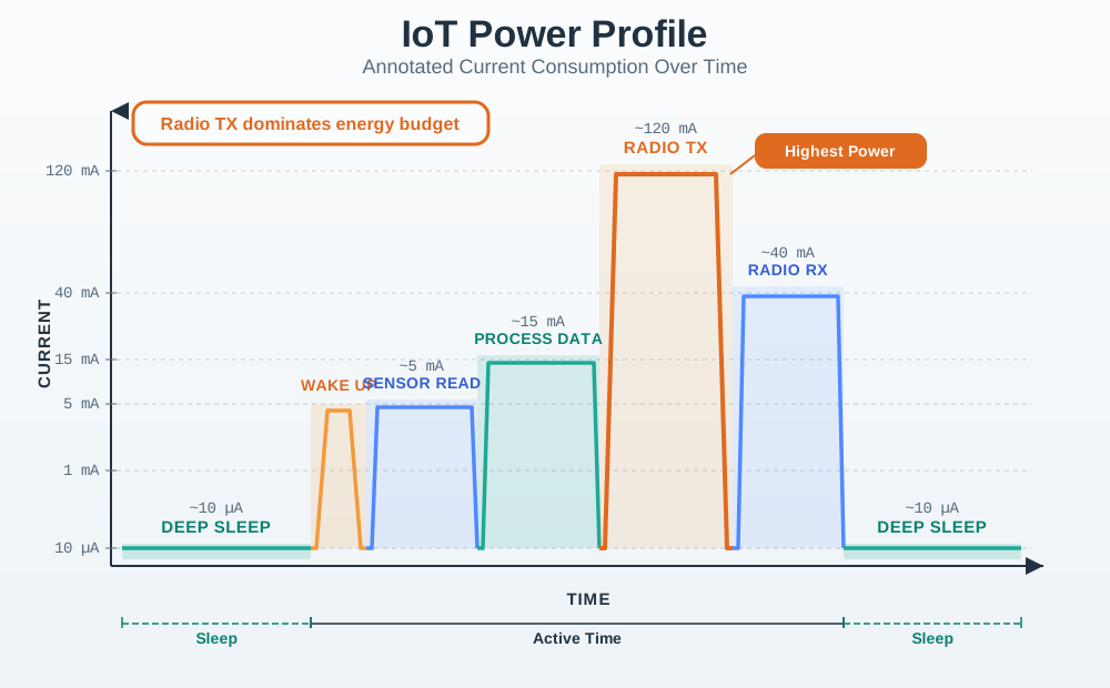
Read the trace as an area problem, not just as a peak-current problem. A 120 mA transmit state that lasts 2 s contributes 240 mA-s; a 10 uA sleep state that lasts 900 s contributes only 0.010 mA x 900 = 9 mA-s. In that cycle, the tall radio block spends more charge than fifteen minutes of sleep. The lab therefore asks for a time-aligned trace before it asks for a battery-life answer.

Intuition only: measure every state the device visits in a full cycle, in order, on the same board you will ship. The largest charge contribution decides where optimization pays off.

The State Ladder

Active radio

WiFi transmit or associate, roughly 150-240 mA on an ESP32. Short but by far the most intense state.

Active compute

CPU running with the radio off, roughly 20-40 mA depending on clock. Sensing and processing live here.

Light sleep

About 0.8 mA with RAM and peripherals retained and a fast wake. A middle resting state.

Deep sleep

About 10 uA with only the RTC alive. The floor that sets life for infrequent reporters.

Overview Knowledge Check

18.23 Build The Measured State Ledger

Capture a full duty cycle and record the measured current and duration of each state, then compute the charge per state as current x duration and sum to a cycle charge. Divide by the cycle time for the average current. The state with the largest charge is where optimization pays.

Worked Example: Report Every 10 Minutes Over WiFi

A bare ESP32 module reports once every 600 s. Measured whole-device states: deep sleep 12 uA; wake and sensor read 40 mA for 120 ms; WiFi associate and transmit 150 mA for 1.5 s.

• WiFi burst: 150 mA x 1.5 s = 225 mA-s.
• Wake and sense: 40 mA x 0.12 s = 4.8 mA-s.
• Deep sleep: 0.012 mA x 598.4 s = 7.2 mA-s.
• Cycle total: 237 mA-s over 600 s, so Iavg = 0.395 mA (395 uA). On a 2000 mAh pack that is about 5060 h, roughly 211 days.

The measurement reveals the surprise: the WiFi burst is 225 of 237 mA-s, about 95% of the cycle charge, while deep sleep is only 3%. For this node, optimizing sleep barely helps; cutting the 1.5 s association cost - a static IP to skip DHCP, a faster connection, or reporting less often - is where the battery is won.

Use the same ledger to test proposed fixes before changing code. If a static IP cuts association from 1.5 s to 0.5 s at the same 150 mA, the WiFi charge falls from 225 to 75 mA-s and the cycle total drops to about 87 mA-s. The average becomes 87 / 600 = 0.145 mA, roughly 2.7 times better than the measured baseline. That is a measurable hypothesis the next lab run can confirm or reject.

Measured Cycle Ledger

State

Measured Current

Duration Per Cycle

Charge (Share)

WiFi associate + TX

150 mA

1.5 s

225 mA-s (95%)

Wake + sense

40 mA

0.12 s

4.8 mA-s (2%)

Deep sleep

12 uA

598.4 s

7.2 mA-s (3%)

Practitioner Knowledge Check

18.24 The Board Is Not The Datasheet

The chip datasheet may promise a 10 uA deep sleep, but a development board rarely delivers it. A typical dev board keeps a USB-to-serial bridge, an always-on voltage regulator with milliamp-scale quiescent current, a power LED, and pull-up resistors alive during sleep. Together these can hold the board at hundreds of microamps to several milliamps in "deep sleep" - a floor that has nothing to do with the processor and everything to do with the board around it.

Rerun the earlier example on such a dev board. Suppose its measured sleep is 10 mA instead of 12 uA. Deep sleep now contributes 10 mA x 598.4 s = 5984 mA-s per cycle, and the cycle total jumps from 237 to about 6214 mA-s. The average current rises to 10.4 mA and the same 2000 mAh pack lasts about 193 h - roughly 8 days instead of 211. Identical firmware, a 26x difference in life, entirely because of the board's sleep floor. That is why you measure the hardware you will ship, disable or remove the bridge and LED for production, and choose a regulator with microamp quiescent current.

The practical test is to isolate loads one at a time while watching the sleep plateau. Remove the power LED and repeat the trace; depower the USB bridge and repeat; then swap the regulator or feed the board after the regulator and repeat. If the floor falls from 10 mA to 0.3 mA after removing debug hardware, then to 25 uA on a bare module, the evidence tells you the firmware was not the limiting factor. The shipping design should preserve the bare-module path and leave the convenience hardware out of the sleep current.

Where The Sleep Floor Hides

USB-serial bridge

An always-powered interface chip can draw milliamps during sleep. Remove or depower it for production.

Regulator quiescent

A high-Iq regulator wastes current continuously. Pick one with microamp quiescent draw.

LEDs and pull-ups

A power LED and stray pull-ups leak milliamps and tens of microamps around the clock.

Retention options

RTC memory and ULP coprocessor raise the floor above the bare deep-sleep number; measure the mode you will use.

Under-the-Hood Knowledge Check

18.25 Summary

This lab applies energy-aware design by measuring current, estimating battery life, comparing operating modes, and validating the effect of firmware and communication changes.

18.26 Key Takeaway

A useful energy lab produces evidence, not just calculations. Measure baseline current, change one policy at a time, compute lifetime impact, and explain any mismatch between estimates and traces.