11  ZRP Hybrid Zone Routing

11.1 Start Simple

Start with devices that have to pass useful data before any fixed network is guaranteed. In ZRP Hybrid Zone Routing, the first question is not the protocol name; it is which neighbors, routes, failure signals, and degraded behaviors you would trust in the field.

11.2 Start With the Local Zone

ZRP starts from a compromise: keep nearby routes ready, but do not flood the whole network until a destination falls outside the local zone. The zone radius turns routing strategy into a design choice.

For IoT teams, that choice balances local speed against control overhead. Start with one node’s neighborhood, decide how far proactive knowledge should reach, and then trace what happens when the destination is just beyond that boundary.

Chapter Roadmap

Use this chapter as a design sequence:

1. First frame why ZRP is hybrid: IARP keeps local zone routes ready while IERP and BRP handle destinations beyond the radius.
2. Then trace the protocol mechanics: local lookup, bordercast, border propagation, zone overlap, route reply, and data transmission.
3. Next tune the radius with the campus and factory numbers, including the 50-85% bordercast savings claim.
4. Finally test degeneration risks, quizzes, the label diagram, and the code challenge.

Checkpoints recap the proof; collapsed sections are deeper references.

In 60 Seconds

Zone Routing Protocol (ZRP) divides networks into overlapping zones of configurable radius (typically 2-3 hops), using proactive routing within zones and reactive discovery between them. Bordercast reduces route discovery overhead by 50-85% compared to pure flooding – zone radius is the critical tuning parameter.

Minimum Viable Understanding

• Zone Routing Protocol (ZRP) divides the network into overlapping zones of configurable radius (typically 2-3 hops), using proactive routing within zones (IARP) and reactive discovery between zones (IERP)
• Bordercast is ZRP’s key optimization: route requests are sent only to zone border nodes rather than flooding the entire network, reducing discovery overhead by 50-85% compared to pure reactive protocols
• Zone radius is the critical tuning parameter: too small (radius=1) degenerates toward pure reactive routing; too large (radius >= network diameter) degenerates toward pure proactive routing with no hybrid benefit

Neighborhood Map Strategy

“I’m confused,” said Sammy the Sensor. “Proactive routing keeps maps of EVERYWHERE (exhausting!). Reactive routing has NO map and asks for directions every time (slow!). Is there a middle ground?”

“YES!” said Max the Microcontroller excitedly. “It’s called Zone Routing Protocol, and it’s like knowing your own neighborhood really well, but using a GPS for trips across town!”

Bella the Battery drew a circle around herself. “See this circle? That’s my ZONE – everything within 2 hops. I know exactly how to reach everyone in my zone (proactive). But for sensors OUTSIDE my zone? I just ask my border friends to pass the question along (reactive)!”

Lila the LED added the best part: “When I need to find someone far away, I don’t shout to the ENTIRE network. I only ask the sensors at the EDGE of my zone – the border nodes. They check THEIR zones, and the question ripples outward efficiently. It’s called BORDERCASTING!”

The Squad’s zone radius guide:

• Radius = 1 hop: Tiny zone, lots of asking around (mostly reactive)
• Radius = 2-3 hops: Sweet spot! Know your neighbors, ask for the rest
• Radius = 10 hops: Zone covers everything – you’re back to proactive mode with all its overhead!

11.3 Learning Objectives

By the end of this chapter, you will be able to:

• Explain ZRP Architecture: Describe how Zone Routing Protocol combines proactive and reactive approaches with its three components (IARP, IERP, BRP)
• Design Zone Configurations: Select appropriate zone radius values for different network characteristics and justify the choice
• Analyze Intra-Zone Routing: Explain proactive table maintenance within each node’s zone and calculate zone size
• Apply Inter-Zone Routing: Demonstrate reactive discovery for destinations outside the zone using bordercast
• Evaluate Hybrid Trade-offs: Assess routing overhead, latency, and scalability trade-offs in ZRP networks
• Compare Protocol Classes: Choose between proactive, reactive, and hybrid protocols for specific scenarios and defend the selection

Quick Check: Campus ZRP Tuning Proof

11.4 Prerequisites

Before diving into this chapter, you should be familiar with:

• Ad Hoc Routing: Proactive (DSDV): Understanding DSDV’s table-driven approach is essential because ZRP uses proactive routing within zones, making DSDV concepts directly applicable to intra-zone routing
• Ad Hoc Routing: Reactive (DSR): Knowledge of DSR’s on-demand route discovery is critical because ZRP employs reactive routing for inter-zone communication, building on DSR’s flooding and route caching mechanisms
• Multi-Hop Fundamentals: Multi-hop networking concepts underpin ZRP’s zone structure, as zone radius is defined in hops and border nodes forward queries across multiple hops
• Networking Basics: Fundamental networking concepts like routing tables, hop counts, and packet forwarding are prerequisites for understanding how ZRP combines proactive and reactive strategies

Key Concepts

• ZRP (Zone Routing Protocol): Hybrid ad hoc routing protocol partitioning the network into zones; proactive within zones, reactive between zones
• Routing Zone: Each node’s local neighborhood within radius ρ hops; routes are maintained proactively within this zone
• Zone Radius (ρ): Number of hops defining the routing zone boundary; large ρ → more proactive overhead; small ρ → more reactive discovery
• IARP (IntraZone Routing Protocol): Proactive component of ZRP maintaining routes within the routing zone
• IERP (InterZone Routing Protocol): Reactive component of ZRP discovering routes to nodes outside the routing zone
• Bordercast: ZRP optimization where route requests are forwarded only to border nodes (at the edge of the zone) rather than flooded
• Zone Overlap: Nodes within ρ hops of each other share zone membership; enables route caching from zone neighbors
• ZRP Trade-off: Optimal ρ exists between all-proactive (ρ=∞) and all-reactive (ρ=1); depends on network size and mobility

11.5 For Beginners: Hybrid Routing (ZRP)

Imagine planning routes in your city. For nearby places (your neighborhood), you keep routes in your head constantly. For distant places (across the city), you only look up directions when needed. Zone Routing Protocol (ZRP) combines both strategies - the best of proactive and reactive routing!

The Goldilocks Protocol:

• Proactive (DSDV): Too much overhead (maintains routes to everywhere continuously)
• Reactive (DSR): Discovery delay for every communication
• Hybrid (ZRP): Just right! Maintains routes only to nearby nodes, discovers distant routes on-demand

How ZRP Works: The Neighborhood Concept

Each node defines a “zone” around itself (like knowing your neighborhood well): - Zone Radius: Distance in hops defining your neighborhood (typically 2-3 hops) - Inside Zone: You maintain routes proactively (like knowing every house on your block) - Outside Zone: You discover routes reactively only when needed (like looking up distant addresses)

Example with Zone Radius = 2:

Node A’s zone includes all nodes within 2 hops: - 1-hop away: Direct neighbors B, C (always know how to reach them) - 2-hops away: Neighbors’ neighbors D, E (proactively maintain routes) - 3+ hops away: F, G, H (discover routes only when needed)

Result: A maintains ~10-12 routes instead of 100 routes (saves 90% memory and overhead!)

Key terms in plain language:

• Zone routing: combine proactive nearby routes with reactive distant discovery, like knowing your neighborhood and using a map for trips across town.
• Zone radius: the local neighborhood size in hops, such as “everyone within 2 hops.”
• Intra-zone routing: proactive routing inside the zone, like knowing all nearby streets.
• Inter-zone routing: reactive routing outside the zone, like looking up directions to another neighborhood.
• Border nodes: nodes at the edge of the zone, like houses on the corner of a block.
• Bordercast: send queries only to border nodes instead of asking the whole network.

The Smart Discovery Process:

When A needs to send to distant node H: 1. Local Check: A checks zone table - “H not in my zone” 2. Bordercast: A sends query to border nodes (D, E) - not full network flood! 3. Border Propagation: D and E check their zones - “Not here either” 4. Zone Overlap: Eventually query reaches zone containing H 5. Local Delivery: That zone delivers to H using proactive routes 6. Reply: Route sent back to A

Comparison:

• DSDV maintains routes to all nodes. It has high idle overhead and high memory use, but no discovery delay.
• DSR maintains no proactive routes. It has low idle overhead, but every new destination needs discovery.
• ZRP maintains only nearby zone routes. It keeps nearby latency low while using reactive discovery for distant nodes.

Zone Radius Selection - The Critical Choice:

Small Zone (radius=1):

• Pros: Low proactive overhead (few nodes), low memory
• Cons: Frequent discoveries (most destinations outside zone)
• Best for: Sparse networks, infrequent communication

Large Zone (radius=5):

• Pros: Most destinations in zone, fewer discoveries
• Cons: High proactive overhead, large routing tables
• Best for: Dense networks, frequent communication

Optimal (radius=2-3):

• Balances both approaches for most IoT networks
• ~10-20 nodes per zone in typical mesh

When to Use ZRP:

Good fit:

• Medium to large IoT networks (100-1000 nodes)
• Clustered topology (sensors grouped around gateways)
• Mixed traffic patterns (frequent local, occasional distant)
• Moderate mobility where zones can still remain useful

Poor fit:

• Very small networks where DSR is simpler
• Very large dense networks where zone maintenance becomes too expensive

Why This Matters for IoT:

Many IoT deployments have clustered communication patterns - sensors talk frequently to nearby devices and their local gateway, but rarely to distant sensors. ZRP perfectly matches this pattern: fast local communication (proactive) + efficient distant communication (reactive) + lower overhead than pure proactive!

Checkpoint: Hybrid Frame

You now know:

• ZRP is the middle path between DSDV’s continuous everywhere table and DSR’s discovery for every new destination.
• The local design question is radius: radius 1 is mostly reactive, radius 2-3 is the usual sweet spot, and radius 10 can become proactive again.
• In the beginner example, a node tracks about 10-12 nearby routes instead of 100 routes, saving about 90% of the local table work.

Related Chapters

Deep Dives:

• Ad Hoc Routing: Proactive (DSDV) - Proactive routing fundamentals
• Ad Hoc Routing: Reactive (DSR) - Reactive routing fundamentals
• Ad-hoc Fundamentals - Ad-hoc network basics

Protocols:

• Multi-Hop Fundamentals - Multi-hop routing concepts
• Routing Fundamentals - General routing
• RPL Routing - IoT-specific routing

Architecture:

• Wireless Sensor Networks - WSN architectures
• DTN and Social Routing - Delay-tolerant approaches

Comparisons:

• Deploying Ad-Hoc Networks - Protocol comparison
• Network Topologies - Topology options

Advanced Topics:

• Ad-hoc Labs and Quiz - Hands-on implementation
• UAV Networks for IoT - Flying ad-hoc networks

Learning:

• Simulations Hub - ZRP simulators
• Network Design - Network testing

The opening sections defined the hybrid idea. The next sections trace which component knows the route, which component searches, and how border nodes bound the query.

11.6 Zone Routing Protocol (ZRP)

Time: ~15 min | Level: Advanced | Unit: P04.C03.U01

Zone Routing Protocol (ZRP) combines proactive and reactive approaches to balance their trade-offs.

11.6.1 ZRP Concept

ZRP divides the network into zones centered on each node:

Alternative View:

Figure 11.1: Zone Routing Protocol diagram showing source node A, one-hop neighbors, two-hop border nodes, proactive IARP links inside the zone, and reactive inter-zone discovery paths beyond the zone boundary.

Figure 11.2: Decision flow showing how ZRP chooses between IARP local delivery, IERP bordercast discovery, and zone-radius retuning when the configured zone is too large or too small.

Figure 11.3: Side-by-side comparison of DSDV, DSR, and ZRP for a 100-node ad hoc IoT network, emphasizing proactive table size, discovery latency, idle overhead, and best-fit scenarios.

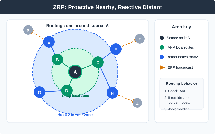
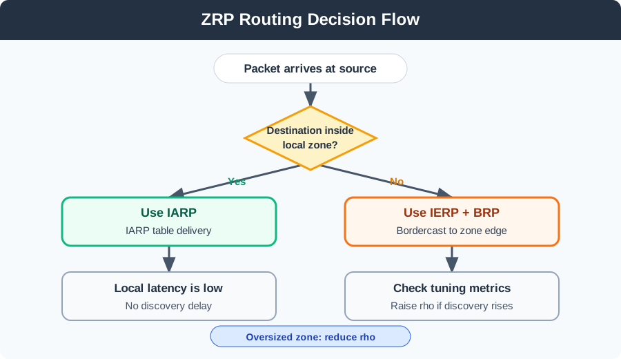
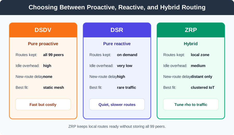
Zone Definitions:

Intra-Zone (Proactive):

Within zone radius, maintain routes proactively using table-driven protocol (like DSDV)

Inter-Zone (Reactive):

Beyond zone, use on-demand route discovery (like DSR)

Zone Radius:

Configurable parameter ρ (rho) defining zone size in hops

Putting Numbers to It

ZRP zone size estimation: In a mesh with average degree d = 5, each extra hop adds another layer of neighbors. A practical estimate is: start with the source node, add the direct neighbors, then add each next hop after accounting for overlap. Worked example:

• rho = 1: about 5 nodes
• rho = 2: about 25 nodes
• rho = 3: can approach 100 nodes in a 100-node network

If rho = 3 already covers nearly the full network, ZRP degenerates toward pure DSDV and loses its hybrid benefit. IoT deployments usually start with rho = 2 or rho = 3, then tune from measured traffic locality.

11.6.2 ZRP Components

Figure 11.4: Block diagram showing the three ZRP components: IARP maintaining proactive intra-zone tables, IERP discovering inter-zone routes on demand, and BRP directing route requests to border nodes.

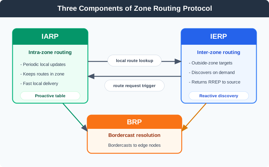
IARP (Intra-zone Routing Protocol):

• Proactive protocol within zone
• Nodes exchange periodic updates
• Maintain routes to all nodes within ρ hops
• Example: Modified DSDV with limited hop count

IERP (Inter-zone Routing Protocol):

• Reactive protocol for distant nodes
• Route requests propagated via border nodes
• Similar to DSR but leverages zone structure

BRP (Bordercast Resolution Protocol):

• Efficient query propagation
• Route requests sent only to zone border nodes
• Reduces flooding overhead

11.6.3 ZRP Operation Example

Scenario: Node A needs to communicate with Node H

Figure 11.5: Sequence diagram showing ZRP inter-zone discovery: source A checks IARP, sends a BRP bordercast to edge nodes, border zones continue the search, and destination H replies through the discovered path.

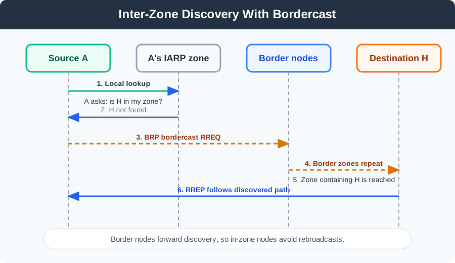
Step-by-Step:

1. Local lookup: A checks IARP table (proactive zone routes)

   • H not within zone radius

2. Bordercast: A sends RREQ to zone border nodes (not full flood)

   • Border nodes: B, C, D

3. Border propagation: Border nodes check their zones

   • If H not found, forward RREQ to their borders

4. Zone overlap: Eventually RREQ reaches zone containing H

   • That zone’s node uses IARP to reach H locally

5. Route reply: RREP sent back to source

6. Data transmission: Source uses discovered route

Smart Campus ZRP Radius

Scenario: A university deploys 200 IoT sensors across a campus for environmental monitoring. Sensors communicate frequently with nearby peers (within buildings) but occasionally need to reach sensors in distant buildings.

Given:

• 200 nodes across 5 buildings
• Average node degree: 6 neighbors per node
• 70% of communication is local (same building)
• 30% of communication is cross-building (distant)
• Battery-powered sensors (energy efficiency critical)

Steps:

1. Estimate nodes per zone radius:
   • ρ=1: ~6 nodes (direct neighbors only)
   • ρ=2: ~6 + (6×5) = 36 nodes (accounting for overlap ~25 nodes)
   • ρ=3: ~75-100 nodes (approaching building-wide coverage)
2. Analyze traffic patterns:
   • 70% local traffic → most destinations should be in-zone
   • Average building has 40 nodes
   • ρ=2 covers ~25 nodes (62% of building) - insufficient
   • ρ=3 covers ~75 nodes (covers full building) - matches traffic pattern
3. Calculate overhead trade-off:
   • ρ=2: Proactive for 25 nodes, reactive for 175 (many discoveries)
   • ρ=3: Proactive for 40 nodes, reactive for 160 (fewer discoveries)
   • Cross-building: 30% traffic × reactive discovery overhead

Result: Zone radius ρ=3 is optimal because: - Covers entire buildings proactively (matches 70% local traffic) - Only cross-building communication (30%) requires reactive discovery - Proactive overhead: 40 entries (acceptable for campus sensors)

Key Insight: Match zone radius to your communication locality. If most traffic is within a certain hop range, set ρ to cover that range proactively. The campus’s building-clustered topology made ρ=3 ideal for intra-building coverage.

Campus Radius Review Record

A ZRP release record should show why the selected radius fits the topology instead of copying a default value. Record traffic locality, typical hop distance, cross-building discovery rate, alarm-latency target, route-table entries, IARP update volume, memory use, battery impact, and the evidence that will trigger retuning, such as zone size above 60 percent of the network, discovery rate above target, mobility churn, or battery drain beyond budget.

Bordercast Route Discovery

Scenario: Node A needs to send critical alarm data to Node H (fire detected). Calculate the route discovery overhead comparing ZRP bordercast versus full network flood (DSR-style).

Given:

• Network: 100 nodes, average degree 5
• Zone radius ρ=2
• Node A has 4 border nodes (B, C, D, E)
• Each border node has 3-4 external connections
• H is 5 hops away from A

Steps:

1. Calculate DSR-style full flood:
   • RREQ flooded to all 100 nodes
   • Each node rebroadcasts once: 100 transmissions
   • Network-wide overhead: 100 RREQ packets
2. Calculate ZRP bordercast:
   • A sends RREQ to 4 border nodes only (not all neighbors)
   • Border nodes check their zones (4 nodes × 25 zone members = 100 lookups, but local)
   • H not found → bordercasting continues from border of border
   • Tier 1: 4 bordercasts
   • Tier 2: 4 borders × 3 external connections = 12 bordercasts
   • Tier 3: H found in zone of tier-2 border node
   • Total: 4 + 12 + local lookup = ~16 transmissions
3. Compare overhead:
   • DSR: 100 transmissions (full flood)
   • ZRP: 16 transmissions (bordercast)
   • Savings: 84% reduction in discovery overhead

Result: ZRP discovered route to H with only 16 messages vs 100 for full flooding.

Key Insight: Bordercast efficiency comes from leveraging zone knowledge - each border node already knows its zone members proactively, so inter-zone discovery only floods between zones, not within them. The larger the zones relative to network size, the greater the savings.

Checkpoint: Route Discovery Mechanics

You now know:

• IARP owns in-zone proactive routes, IERP owns out-of-zone discovery, and BRP directs route requests to border nodes.
• The campus example uses 200 nodes across 5 buildings with 70% local and 30% cross-building traffic to justify radius 3.
• In the fire-alarm discovery example, bordercast uses about 16 transmissions instead of 100 full-flood transmissions, an 84% reduction.

The route trace proves ZRP can search efficiently. The remaining design work is deciding when that efficiency justifies a larger local zone.

11.6.4 ZRP Zone Radius Selection

The zone radius ρ critically affects performance:

Radius trade-off guide:

• rho = 1: low proactive overhead, high reactive overhead. Best for sparse networks and infrequent communication.
• rho = 2: low-to-medium proactive overhead, medium reactive overhead. This is the usual starting point for IoT deployments.
• rho = 3: medium proactive overhead, lower reactive overhead. Good for dense networks with frequent local traffic.
• rho = 4: high proactive overhead, low reactive overhead. Use only in very dense, stable networks.
• rho = 5: very high proactive overhead, very low reactive overhead. Use only when the topology is static and local traffic dominates.

Small Zone Radius (ρ=1):

• Low proactive overhead (few nodes in zone)
• High reactive overhead (frequent inter-zone queries)
• Good for sparse communication

Large Zone Radius (ρ=4-5):

• High proactive overhead (many nodes in zone)
• Low reactive overhead (most destinations in zone)
• Good for frequent communication

Optimal Radius:

• Depends on network size, topology, traffic patterns
• Typically ρ = 2-3 for IoT deployments
• Adaptive schemes adjust ρ based on observed traffic

11.6.5 When ZRP Stops Being Hybrid

ZRP is not automatically better than proactive or reactive routing. Its benefit exists only while the configured zone boundary matches the network’s topology and traffic pattern.

• Oversized zones: if the radius approaches the network diameter, every node is in-zone, IERP stops doing useful work, and ZRP behaves like DSDV with extra complexity.
• Undersized zones: if most destinations are outside the zone, local route tables are cheap but nearly every useful packet triggers reactive discovery.
• Moving borders: mobility changes zone membership, border-node identity, cached routes, and IARP freshness at the same time.
• Bad bordercast: if BRP falls back to full flooding or misses true border nodes, the measured overhead no longer matches the design record.

11.6.6 ZRP Performance Characteristics

Use the performance questions to separate three ideas that are easy to blur: how many routes IARP maintains inside the zone, how often IERP has to search beyond the zone, and whether BRP is reducing discovery work instead of silently becoming a flood.

Knowledge Check

Test your understanding of these architectural concepts.

Hybrid Routing With ZRP

11.7 ZRP Zone Radius Explorer

Estimate how zone radius affects proactive vs reactive overhead in ZRP:

viewof zone_radius = Inputs.range([1, 6], {value: 2, step: 1, label: "Zone radius ρ (hops)"})
viewof avg_degree = Inputs.range([2, 10], {value: 5, step: 1, label: "Average node degree"})
viewof total_nodes = Inputs.range([20, 300], {value: 100, step: 10, label: "Total network nodes"})

{
  // Zone size estimate: sum of geometric series
  let zone_size = 1;
  let layer = 1;
  for (let i = 1; i <= zone_radius; i++) {
    layer = (i === 1) ? avg_degree : layer * (avg_degree - 1);
    zone_size += Math.min(layer, total_nodes - zone_size);
  }
  zone_size = Math.min(zone_size, total_nodes);
  
  const border_pct = (zone_size / total_nodes) * 100;
  const proactive_mb = (total_nodes * 240 * zone_size * 50) / 1e6; // 50B/entry, 240 updates/hr
  const reactive_pct = Math.max(0, 100 - border_pct);
  const reactive_mb = (total_nodes * 30 * (reactive_pct/100) * total_nodes * 60) / 1e6;
  const total_mb = proactive_mb + reactive_mb;
  
  const pure_dsdv = (total_nodes * 240 * total_nodes * 50) / 1e6;
  const savings_pct = ((pure_dsdv - total_mb) / pure_dsdv * 100);
  
  const status = zone_size >= total_nodes * 0.6 ? 'Too large (→ DSDV)' : 
                 zone_size <= total_nodes * 0.1 ? 'Too small (→ DSR)' : 'Optimal range';
  
  return html`
    <div style="display:grid;grid-template-columns:repeat(auto-fit,minmax(10rem,1fr));gap:0.7rem;margin:1rem 0">
      <div style="background:#eaf4fb;border-left:4px solid #3498DB;padding:0.8rem;border-radius:4px;min-width:0">
        <div style="font-size:0.8rem;color:#555">Zone size</div>
        <div style="font-size:1.5rem;font-weight:bold;color:#2C3E50">${zone_size} nodes</div>
        <div style="font-size:0.75rem;color:#777">${border_pct.toFixed(0)}% of network</div>
      </div>
      <div style="background:#fef9e7;border-left:4px solid #E67E22;padding:0.8rem;border-radius:4px;min-width:0">
        <div style="font-size:0.8rem;color:#555">Proactive overhead</div>
        <div style="font-size:1.5rem;font-weight:bold;color:#2C3E50">${proactive_mb.toFixed(0)} MB/hr</div>
      </div>
      <div style="background:#eafaf1;border-left:4px solid #16A085;padding:0.8rem;border-radius:4px;min-width:0">
        <div style="font-size:0.8rem;color:#555">vs pure DSDV</div>
        <div style="font-size:1.5rem;font-weight:bold;color:#2C3E50">${savings_pct.toFixed(0)}% saved</div>
      </div>
      <div style="background:${status.includes('Optimal') ? '#eafaf1' : '#fdf2f8'};border-left:4px solid ${status.includes('Optimal') ? '#16A085' : '#E74C3C'};padding:0.8rem;border-radius:4px;min-width:0">
        <div style="font-size:0.8rem;color:#555">Assessment</div>
        <div style="font-size:0.95rem;font-weight:bold;color:#2C3E50">${status}</div>
      </div>
    </div>
    <p style="font-size:0.9rem;color:#555">ρ=${zone_radius} covers ${zone_size}/${total_nodes} nodes (${border_pct.toFixed(0)}%). Proactive: ${proactive_mb.toFixed(0)} MB/hr for zone routes. Pure DSDV would be ${pure_dsdv.toFixed(0)} MB/hr. Target zone coverage: 20-50% of network for true hybrid behavior.</p>
  `;
}

Checkpoint: Radius Tuning

You now know:

• Increasing radius shifts cost from reactive discovery into proactive tables; it cannot make both costs disappear.
• The explorer frames true hybrid behavior as roughly 20-50% zone coverage, while a zone above 60% of the network is a warning sign.
• The 150-sensor campus worked example chooses rho = 2 when 43.75% reactive traffic is acceptable and rho = 3 costs 3.3x more overhead.

The tuning examples show that ZRP is a measured configuration. The next section asks what it buys IoT deployments once that configuration is in range.

11.8 ZRP Benefits for IoT

Time: ~8 min | Level: Intermediate | Unit: P04.C03.U02

Advantages:

• Balanced overhead: Combines benefits of proactive and reactive
• Reduced flooding: Bordercasting more efficient than full flood
• Low latency for nearby: Proactive routes to local nodes
• Scalable: Reactive component handles distant nodes efficiently
• Configurable: Adjust zone radius to optimize for specific scenarios

Disadvantages:

• Complexity: More complex than pure proactive or reactive
• Overhead: Still maintains proactive routes (better than DSDV, worse than DSR for sparse traffic)
• Configuration: Optimal zone radius difficult to determine
• Border management: Identifying and maintaining border nodes adds overhead

Best For:

• Medium to large IoT networks (100-1000 nodes)
• Heterogeneous traffic: frequent local, occasional distant communication
• Cluster-based IoT topologies (sensors clustered around gateways)
• Hierarchical networks with localized communication patterns

Cross-Hub Connections

This chapter connects to multiple learning resources:

Simulations Hub:

• Network Simulations - Interactive ZRP zone visualization and bordercast simulation tools

Videos Hub:

• Routing Protocol Videos - Visual explanation of ZRP operation and zone configuration

Quizzes Hub:

• Ad-hoc Routing Quizzes - Self-assessment on hybrid routing concepts

Knowledge Gaps Hub:

• Common Routing Misconceptions - Addressing confusion between proactive, reactive, and hybrid approaches

ZRP Radius Trade-offs

Misconception: Students often believe that increasing zone radius always improves ZRP performance by reducing route discovery overhead.

Reality: Zone radius selection involves critical trade-offs:

Zone Radius Too Large (ρ=5-7):

• Risk: high proactive overhead from maintaining routes to 50-100 nodes continuously.
• Risk: excessive update traffic as periodic routing updates flood the zone.
• Risk: large routing tables on resource-constrained IoT nodes.
• Risk: the protocol approaches pure DSDV overhead and loses its hybrid purpose.

Zone Radius Too Small (ρ=1):

• Risk: frequent reactive discoveries because most destinations are outside the zone.
• Risk: high bordercast overhead from constant route requests.
• Risk: increased latency because even nearby nodes may require discovery.
• Risk: the protocol approaches pure DSR behavior and loses its hybrid purpose.

Optimal Zone Radius (ρ=2-3):

• Benefit: balances proactive maintenance for nearby nodes with reactive discovery for distant nodes.
• Benefit: keeps latency low for frequent local communication inside the zone.
• Benefit: discovers occasional distant destinations efficiently through bordercast.
• Benefit: matches clustered IoT traffic, where sensors often report through a nearby gateway.

The Math: In a mesh network with average degree d=5: - ρ=1: ~5 nodes in zone (very reactive) - ρ=2: ~10-15 nodes in zone (balanced) ← Optimal - ρ=3: ~25-50 nodes in zone (mostly proactive) - ρ=4: ~75-125 nodes in zone (approaching DSDV overhead)

Key Insight: ZRP’s advantage comes from matching zone size to communication patterns, not maximizing zone size. Analyze your network’s traffic locality before choosing ρ!

11.9 Visual Reference Gallery

Visual: Ad Hoc Network Schematic

Schematic of an ad hoc network showing self-organizing wireless nodes

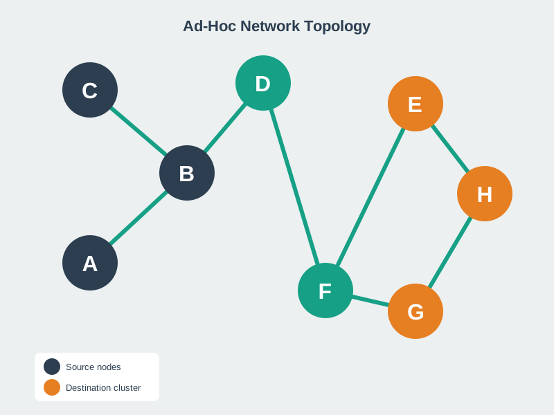
This diagram illustrates the fundamental structure of ad hoc networks where ZRP operates, showing how nodes organize themselves into a mesh without centralized control.

Ad Hoc Routing Protocols

Overview of ad hoc routing protocol categories

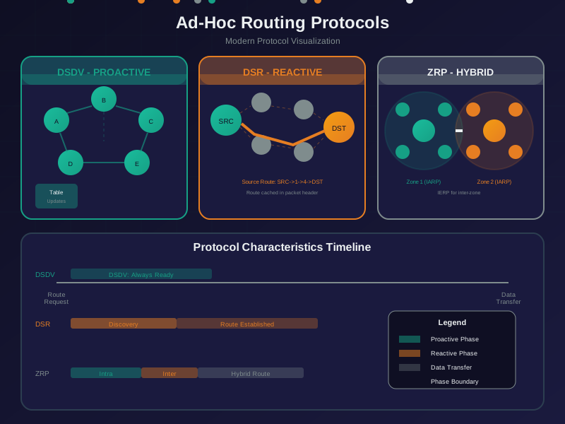
This visualization shows the taxonomy of ad hoc routing protocols, positioning ZRP as the hybrid approach that combines proactive and reactive strategies.

Visual: Ad Hoc Network Architecture

Ad hoc network architecture and connectivity patterns

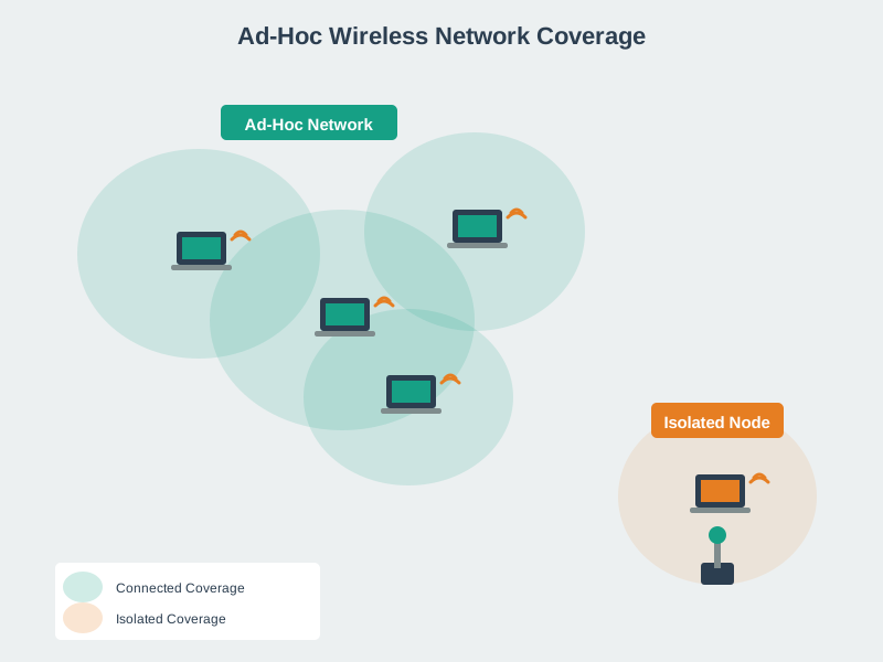
A geometric view of ad hoc network architecture, emphasizing the zone-based structure that ZRP leverages for efficient routing.

ZRP Zone Radius for Campus

Scenario: University campus deploys 150 IoT sensors for environmental monitoring. Calculate optimal ZRP zone radius based on traffic patterns and topology.

Given:

• 150 sensor nodes across 5 buildings
• Building-local traffic: 75% (sensors within same building)
• Cross-building traffic: 25% (sensors to other buildings)
• Average node degree: 5 neighbors
• Typical intra-building path: 2-3 hops
• Inter-building path: 6-8 hops
• Data reporting: Every 2 minutes per sensor

Steps:

1. Calculate zone sizes for different radii:

   • ρ=1: ~5 nodes (direct neighbors only)
   • ρ=2: ~5 + (5 × 4) = 25 nodes (neighbors of neighbors)
   • ρ=3: ~5 + 20 + 60 = 85 nodes (approaching building-wide)
   • ρ=4: ~120 nodes (exceeds single building)

2. Analyze traffic locality:

   • 75% traffic within building → Want most building covered proactively
   • Average building: 30 sensors
   • Target: ρ covers ≥80% of building sensors

3. Calculate proactive overhead for each ρ:

   ρ=2 (25 nodes/zone):

   • Proactive updates: Every 15s = 240/hour
   • Per node: 24 routes × 50 bytes = 1,200 bytes
   • Per node hourly: 240 × 1,200 = 288 KB
   • Network: 150 × 288 KB = 43.2 MB/hour

   ρ=3 (85 nodes/zone):

   • Per node: 84 routes × 50 bytes = 4,200 bytes
   • Per node hourly: 240 × 4,200 = 1,008 KB
   • Network: 150 × 1,008 KB = 151.2 MB/hour

4. Calculate reactive overhead for each ρ:

   ρ=2 (25% of building proactive, 75% + all inter-building reactive):

   • Intra-building reactive: 75% × 25% uncovered = 18.75% of traffic
   • Inter-building reactive: 25% of traffic
   • Total reactive: 43.75% of traffic
   • Discoveries/hour: 150 sensors × 30 pkt/hr × 0.4375 = 1,969 discoveries
   • Bordercast cost: ~30 nodes per discovery × 60 bytes = 1,800 bytes
   • Reactive overhead: 1,969 × 1,800 = 3.54 MB/hour

   ρ=3 (full building proactive, only inter-building reactive):

   • Reactive: 25% of traffic
   • Discoveries/hour: 150 × 30 × 0.25 = 1,125
   • Reactive overhead: 1,125 × 1,800 = 2.03 MB/hour

5. Total overhead comparison:

   Overhead comparison:

   • rho = 2: proactive overhead is 43.2 MB/hr, reactive overhead is 3.54 MB/hr, total overhead is 46.74 MB/hr, and coverage is about 57% proactive.
   • rho = 3: proactive overhead is 151.2 MB/hr, reactive overhead is 2.03 MB/hr, total overhead is 153.23 MB/hr, and coverage is about 85% proactive.

6. Decision analysis:

   • ρ=2: Lower overhead (46.74 MB) but 43.75% traffic requires discovery (delay)
   • ρ=3: 3.3× higher overhead but 75% traffic is instant (no discovery)
   • Trade-off: Is 106 MB/hour extra overhead worth eliminating discovery for 75% of traffic?

7. Calculate cost per eliminated discovery:

   • Extra overhead: 153.23 - 46.74 = 106.49 MB/hour
   • Discoveries eliminated: 1,969 - 1,125 = 844/hour
   • Cost: 126 KB per eliminated discovery

Result: Choose ρ=2 (zone radius = 2 hops)

Rationale:

• 75% intra-building traffic mostly covered (2-3 hop paths, zone covers 2 hops)
• Overhead 3.3× lower than ρ=3
• 43.75% reactive traffic acceptable for environmental monitoring (not latency-critical)
• Building-scale zones align naturally with campus physical topology

Alternative: If latency were critical (fire alarms), choose ρ=3 despite 3× overhead.

Key Insight: Optimal zone radius depends on traffic locality pattern. Match zone size to your network’s natural clusters (buildings, floors, departments). Oversizing zones (ρ → network diameter) degenerates to pure proactive with no hybrid benefit.

ZRP Zone Radius Selection

Choose zone radius based on measurable network characteristics and application requirements.

Selection factors:

• Small zone (rho = 1-2): best for 20-50 nodes, sparse local traffic below 50%, network diameter above 10 hops, latency tolerance above 1 second, and tight battery budgets. It typically covers 5-10% of the network.
• Medium zone (rho = 2-4): best for 50-200 nodes, moderate traffic locality of 50-80%, network diameter of 6-10 hops, latency targets of 200-1000 ms, and moderate overhead budgets. It typically covers 20-40% of the network.
• Large zone (rho = 4-6): best for 200-1000 nodes only when local traffic is above 80%, network diameter is 4-6 hops, latency must stay below 200 ms, and nodes have enough power budget. It can cover 60-80% of the network, so watch for proactive degeneration.

Zone Radius Selection Algorithm:

def select_optimal_zone_radius(
    network_size: int,
    avg_neighbors: int,
    traffic_locality: float,  # 0.0-1.0, fraction of traffic within 3 hops
    latency_requirement_ms: int,
    overhead_budget_mb_per_hour: float
) -> int:
    """
    Calculate optimal ZRP zone radius.

    Returns: Recommended zone radius (hops)
    """

    # Estimate zone size for each radius
    zone_sizes = {
        1: avg_neighbors,
        2: avg_neighbors * (avg_neighbors - 1),
        3: avg_neighbors * (avg_neighbors - 1) ** 2,
        4: avg_neighbors * (avg_neighbors - 1) ** 3,
    }

    # Calculate overhead for each radius
    UPDATE_SIZE_BYTES = 50
    UPDATES_PER_HOUR = 240  # every 15s

    overheads = {}
    for radius, zone_size in zone_sizes.items():
        # Proactive overhead
        proactive = network_size * zone_size * UPDATE_SIZE_BYTES * UPDATES_PER_HOUR / 1e6  # MB

        # Reactive overhead (simplified)
        reactive_fraction = max(0, 1 - (zone_size / network_size))
        reactive = reactive_fraction * network_size * 30 * 1800 / 1e6  # MB (30 pkt/hr/node)

        total = proactive + reactive
        overheads[radius] = total

        # Check if within budget
        if total > overhead_budget_mb_per_hour:
            continue

        # Check latency coverage
        coverage = zone_size / network_size
        if coverage >= traffic_locality:  # Most local traffic covered proactively
            # Check latency requirement
            discovery_latency = 150  # ms (typical bordercast)
            if discovery_latency * (1 - coverage) < latency_requirement_ms * 0.2:  # 20% budget
                return radius

    # Fallback: Choose smallest radius within overhead budget
    for radius in sorted(overheads.keys()):
        if overheads[radius] <= overhead_budget_mb_per_hour:
            return radius

    return 1  # Minimum zone

Example Application:

optimal_radius = select_optimal_zone_radius(
    network_size=150,
    avg_neighbors=5,
    traffic_locality=0.75,  # 75% local
    latency_requirement_ms=500,
    overhead_budget_mb_per_hour=60
)
# Returns: 2 (for smart campus scenario above)

Tuning Rules:

1. Start conservative: Begin with ρ = 2, measure actual traffic locality
2. Monitor overhead: If overhead <50% of budget, consider ρ+1
3. Track discovery rate: If >20% of packets require discovery, consider ρ+1
4. Watch for degeneration: If zone_size > 60% of network, reduce ρ (becoming pure proactive)

Key Insight: Zone radius is not a fixed protocol parameter - it should be dynamically tuned based on observed traffic patterns and network density.

Overlarge ZRP Zones

The Mistake: Configuring ZRP with zone radius ρ ≥ (network diameter / 2), causing hybrid protocol to behave like pure DSDV with all its overhead but none of ZRP’s benefits.

Real-World Example: A 2021 industrial IoT deployment set ZRP zone radius to ρ=8 in a 20-node factory network with 6-hop diameter. After 2 months: - Routing overhead: 95 MB/hour (expected: 30 MB/hour) - Discovery latency: Still 200ms average (expected: <50ms for local) - Battery life: 45% worse than DSDV-only deployment

Root Cause Analysis:

1. Zone radius vs network diameter:
   • ρ=8, network diameter=6 hops
   • Zone covers entire network! (8 hops ≥ 6-hop max distance)
2. IARP behavior (intra-zone proactive):
   • Each node maintains routes to ALL 19 other nodes proactively
   • This is identical to DSDV (pure proactive)
3. IERP behavior (inter-zone reactive):
   • No inter-zone traffic exists (all destinations within zone)
   • IERP component never used (wasted complexity)
4. Bordercast optimization:
   • Border nodes = nodes with neighbors outside zone
   • With ρ ≥ diameter, zero border nodes (everyone’s zone covers network)
   • Bordercast benefit: 0%

Quantified Waste:

ZRP (ρ=8) vs DSDV:

• Overhead: Both maintain 19 routes per node → Identical 95 MB/hour
• Complexity: ZRP has 3 protocol components (IARP, IERP, BRP) vs DSDV’s 1
• Memory: ZRP stores zone member lists + route tables vs DSDV’s single table
• CPU: ZRP runs 3 protocols vs 1

Result: ZRP with oversized zone is strictly worse than DSDV - same overhead, more complexity, more bugs, more maintenance.

How to Detect Oversized Zones:

Monitor these metrics - if ALL are true, zone is too large:

def is_zone_oversized(zone_radius, network_diameter, zone_size, network_size):
    """Returns True if zone radius should be reduced."""
    return all([
        zone_radius >= network_diameter / 2,  # Zone covers >50% of max distance
        zone_size > 0.6 * network_size,       # Zone covers >60% of nodes
        reactive_discovery_rate < 0.05        # <5% of traffic needs discovery
    ])

Correct Configuration for Factory Example:

• Network: 20 nodes, diameter=6 hops
• Optimal ρ: 2-3 hops (covers ~10-15 nodes = 50-75% of network)
• Result:
  • Proactive: 10-15 routes per node (vs 19 in oversized)
  • Reactive: 5-10 routes discovered on-demand
  • Overhead reduction: 55% (from 95 MB/hr to 43 MB/hr)

Design Rules:

1. Maximum zone radius: ρ_max = min(diameter/2, sqrt(network_size)/2)
   • For 20-node, 6-hop network: min(3, sqrt(20)/2) = min(3, 2.2) = 2 hops
2. Zone size constraint: Zone should cover 30-50% of network
   • For 20 nodes: Target 6-10 nodes/zone → ρ=2-3 with avg_degree=5
3. Reactive traffic target: 20-40% of traffic should require inter-zone discovery
   • If <10%, zone too large (degenerating to proactive)
   • If >60%, zone too small (degenerating to reactive)

Measured Impact of Right-Sizing (Factory Fix):

• Before (ρ=8): Overhead 95 MB/hr, battery 4.2 months, identical to DSDV
• After (ρ=2): Overhead 43 MB/hr, battery 9.1 months, 55% savings, true hybrid behavior
• Result: 2.2× battery life extension by fixing single configuration parameter

Key Lesson: ZRP’s benefit comes from the hybrid behavior - proactive for common local routes, reactive for rare distant routes. Oversizing zones kills this benefit. Always validate that 20-40% of traffic requires inter-zone discovery; otherwise, reduce zone radius or switch to pure DSDV (simpler).

Checkpoint: Degeneration Risks

You now know:

• Oversized zones make IERP idle and BRP useless because every destination is already inside the proactive zone.
• The factory example shows the failure mode: rho = 8 in a 20-node, 6-hop network produced 95 MB/hour overhead before right-sizing cut it to 43 MB/hour.
• A healthy design keeps some inter-zone discovery alive, with the chapter’s target range of 20-40% of traffic.

With the risks named, the final quizzes check component names, route-discovery order, and the right action from routing state.

Interactive Quiz: Match Concepts

Interactive Quiz: Sequence the Steps

Common Pitfalls

Choose ZRP Radius by Performance

The optimal zone radius ρ depends on network density, mobility, and traffic pattern. Setting ρ too large causes excessive proactive overhead; ρ too small eliminates the benefit of local pre-computed routes. Use analytical models or simulation to find the optimal ρ for your specific deployment scenario.

ZRP Zones Change With Mobility

As nodes move, the composition of each node’s routing zone changes. Nodes entering and leaving zones require updating the IARP routing tables. High mobility causes frequent zone membership changes and associated overhead — ZRP performs worst in high-mobility scenarios where zones are unstable.

3. Not Implementing Bordercast Correctly

ZRP’s bordercast reduces flooding by sending inter-zone route requests only to border nodes. Implementing full flooding instead of bordercast eliminates ZRP’s primary advantage over pure reactive routing. The bordercast mechanism requires identifying border nodes — nodes at exactly ρ hops from the source.

Tune Before Comparing ZRP

ZRP comparisons are only fair when ρ is tuned to the specific scenario. Comparing ZRP with ρ=1 (effectively pure reactive) to DSDV in a dense, low-mobility network makes ZRP appear worse than a properly configured ZRP would be. Always tune the hybrid parameter before comparing to pure alternatives.

Label the Diagram

Code Challenge

11.10 Summary

This chapter covered ZRP (Zone Routing Protocol) as a hybrid routing approach for ad hoc networks:

• Hybrid Architecture: ZRP combines proactive routing within local zones (IARP) and reactive discovery between distant zones (IERP) to balance overhead and latency
• Zone-Based Design: Each node defines a routing zone with configurable radius ρ, maintaining proactive routes to all nodes within ρ hops while using on-demand discovery beyond
• Protocol Components: IARP handles intra-zone routing using table-driven updates, IERP manages inter-zone reactive discovery, and BRP enables efficient bordercast query propagation
• Zone Radius Selection: Critical parameter ρ determines trade-off between proactive overhead (grows with larger zones) and reactive discovery frequency (increases with smaller zones)
• Bordercast Optimization: Route requests sent only to zone border nodes rather than full network flooding, significantly reducing discovery overhead compared to pure reactive protocols
• Performance Characteristics: ZRP achieves low latency for nearby destinations (proactive), scalable distant communication (reactive), and reduced flooding overhead (bordercasting)
• Optimal Configuration: Typical zone radius ρ = 2-3 hops balances proactive maintenance costs with reactive discovery needs, though optimal value depends on network size, density, and traffic patterns

11.11 What’s Next

• Revisit proactive routing DSDV: DSDV Proactive Routing
• Study reactive routing DSR: DSR Fundamentals and Route Discovery
• Explore DTN for disconnected networks: DTN Store-Carry-Forward
• Learn about ad hoc network applications: Ad-Hoc Network Applications
• Compare ad hoc routing deployment choices: Deploying Ad-Hoc Networks

11.12 Key Takeaway

ZRP combines proactive routing inside a local zone with reactive discovery beyond it. The zone radius is the main tradeoff: small zones reduce overhead, while larger zones improve immediate route knowledge.