25 Digital Twin Concepts and Scenario Assessment
One of two parts on digital twin assessment and practice – the other is Lab: Build a Digital Twin. This part tests conceptual understanding of digital twin architecture through scenario-based questions: synchronization cadence, DTDL properties versus telemetry, conflict resolution, and graph-based relationship modeling.
25.1 Start Simple
Start with one decision that would be safer if a live model stayed aligned with the physical system. In Lab: Build a Digital Twin, the practical question is what state must be synchronized, who acts on it, and what evidence proves the twin is still fit to use.
25.2 Learning Objectives
By the end of this chapter, you will be able to:
- Assess your understanding of digital twin concepts through comprehensive quizzes
- Analyze complex scenarios requiring architectural decision-making
- Build a functional digital twin system using ESP32 and sensors
- Implement bidirectional synchronization between physical and digital entities
- Extend the lab with predictive analytics and anomaly detection features
If you only have 10 minutes, focus on these essentials:
- Digital twins differ from digital shadows by enabling bidirectional data flow – not just monitoring, but also control (Quiz Question 1)
- Edge aggregation is usually required at high volume – sending raw data from hundreds of machines directly to the cloud is impractical (Quiz Question 2)
- The lab demonstrates four core concepts: bidirectional sync, state history via circular buffers, trend-based prediction, and twin-side intelligence
- Start simple: Begin with telemetry mirroring and alerts, then add ML prediction as historical data accumulates
Come back for the full lab when you have 45+ minutes of hands-on time.
This assessment lab has two jobs: test the concept, then make you build the loop.
- First you define the twin as a control claim: state must be fresh, model assumptions must be explicit, and commands must stay bounded.
- Then the quizzes and scenarios pressure-test architecture choices such as edge aggregation, graph relationships, stale data, and conflict handling.
- Next the ESP32 lab turns those ideas into a seven-step synchronization cycle with sensor reads, mirrored state, history, prediction, and LED commands.
- Finally the production and ROI sections ask whether the twin is worth operating once failure data, bandwidth, ownership, and prediction accuracy are included.
Checkpoints mark the main decision points. Deep-dive and collapsed sections are useful references, but the main path is the claim, the evidence, the lab, and the production review.
25.3 Overview: A Twin Is A Control Claim
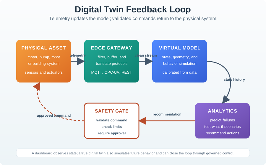
A digital twin is more than a live chart. It claims that the digital model is fresh enough, accurate enough, and trusted enough to influence the physical system through decisions or commands.
This lab should therefore prove more than sensor display. It should show the telemetry source, sync cadence, stale-data rule, model assumption, command path, and the evidence that the physical device responded as intended.
Before running the ESP32 exercise, write the claim in one sentence: for this DHT22, LED, and button circuit, at this sync interval, the twin mirrors temperature and humidity, keeps a bounded state history, predicts the next few cycles, and sends only the LED command that the lab rule permits. That sentence defines what the lab is allowed to prove. It also keeps the exercise from drifting into a generic dashboard demo where every serial print looks convincing but no one can say whether the twin is trustworthy enough to act.
The evidence you collect should follow the control loop. A useful run record ties each sensor read to a timestamp, a mirrored twin state, a history-buffer update, a prediction, a command decision, and a visible physical result. If the DHT22 read fails, the record should say whether the twin reused last-known values or marked the state stale. If the button toggles the LED through twin logic, the record should show the physical input, digital decision, and physical output as one traceable chain.
This is the same discipline used in larger twins, only at lab scale. A building twin may use BACnet points and a BMS instead of an ESP32, and a factory twin may use OPC UA, MQTT, or a historian instead of Serial Monitor output, but the claim is still the same: the model state is current enough, the decision rule is bounded enough, and the physical response is verified enough for this specific action.
25.4 Twin Evidence Record
For each lab run, record the physical entity, sensor inputs, twin state, update interval, edge or cloud responsibility, prediction or anomaly rule, command intent, actuator result, operator owner, and retest trigger.
The useful decision is not simply whether the twin runs. The useful decision is whether the twin is ready for this equipment, this sync delay, this data quality, this control boundary, and this recovery path.
Use a small evidence table while you run the Wokwi circuit. At minimum, capture the run id, sketch version, wiring pins, sync interval, DHT22 reading, `lastSyncTime`, `syncLatencyMs`, circular-buffer count, alert thresholds, predicted temperature, command reason, LED state before and after the command, and any manual observation from the simulator. The table does not need to be elaborate. Its job is to make every pass/fail decision reviewable after the serial log scrolls away.
Separate normal behavior from exception behavior. A normal run proves that the twin mirrors state and commands the LED when the threshold rule is met. An exception run proves that the twin handles failed reads, delayed sync, stale state, or a manual button event without pretending the model is more current than it is. If you add the network-simulation challenge, record both the local buffered readings and the replay rule used when connectivity returns, because replay order can change the average, trend, and alert history.
For a production transfer, replace the lab names with real ownership boundaries. The physical entity becomes a pump, room, robot, or machine. The Serial Monitor becomes a historian, dashboard, alarm log, or work-order record. The LED command becomes a relay, setpoint, recommendation, or operator approval step. The same evidence record should still answer who owns the data, who owns the command, what freshness budget was accepted, and what observation proves the command reached the physical world.
25.5 Prove Twin State Freshness
Network delay, sensor drift, missing packets, model updates, and local buffering all create gaps between physical state and twin state. A mature twin labels those gaps instead of hiding them behind a smooth display.
Edge gateways reduce raw data volume by summarizing, filtering, and forwarding exceptions, but they also become part of the proof chain. The lab record should show what the edge kept, what it sent, and how the cloud twin knows when state is stale.
In the sketch, state drift can come from several places. The DHT22 can return `NaN`, the two-second sync loop can be delayed by other work, the circular buffer can overwrite older evidence, and the LED state can change before the twin has printed a full status block. Those are not just coding details. They are the local version of the same problems production twins face when gateways batch data, message brokers redeliver retained state, historians downsample telemetry, or operators change an asset outside the twin workflow.
The technical safeguard is to treat freshness as data, not as an assumption. A twin state should carry the source timestamp, arrival timestamp, sequence or sync count, model version, command id, and confidence or staleness label. Commands should be idempotent where possible, meaning the same command can be replayed without creating a second unintended physical action. When state is replayed after an outage, the twin should apply it in order or explicitly mark it as historical so old readings do not overwrite newer physical reality.
The lab's simple prediction rule is deliberately easy to inspect: current temperature plus recent trend times a horizon. That transparency is useful for learning, but it does not make the prediction authoritative. The prediction is only safe to act on when the input window is valid, the threshold has a defined owner, the command path is bounded, and the physical result can be checked. In production, an ML model, physics model, or simulation engine needs the same guardrails: versioned inputs, drift monitoring, fallback behavior, and a clear rule for when a human must approve the next action.
Key Concepts
- Digital Twin Assessment Criteria: Synchronization fidelity, model accuracy, prediction performance, and system response time
- State Divergence Metric: Quantified difference between digital twin state and physical entity state; acceptable bounds depend on application
- Simulation Accuracy: How closely the digital twin’s simulated behavior matches actual physical entity behavior
- Lab Scenario: Controlled test case evaluating specific digital twin capabilities (state sync, prediction, anomaly detection)
- Data Quality Assessment: Evaluating completeness, accuracy, and timeliness of sensor data feeding the digital twin
- KPI (Key Performance Indicator): Measurable metric tracking digital twin effectiveness; e.g., prediction error, sync latency, uptime
- Regression Testing: Verifying that digital twin model updates do not degrade previously working capabilities
- Visualization Assessment: Evaluating whether the digital twin’s visual representation accurately conveys physical entity state
25.6 Introduction
This chapter combines assessment and practice. The first half tests your conceptual understanding of digital twin architecture through scenario-based questions covering synchronization, conflict resolution, data modeling, and platform selection. The second half provides a hands-on lab where you build a working digital twin on an ESP32 microcontroller, implementing the same patterns used in industrial systems – at a scale suitable for learning.
Whether you are preparing for an exam or want practical experience, this chapter bridges theory and implementation.
25.7 Digital Twin Maturity Levels
Before diving into the assessment, review the maturity progression from simple monitoring to full digital twin capability. This framework appears repeatedly in the quiz questions and the lab.
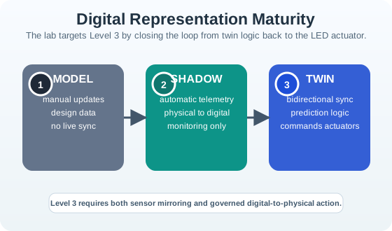
Key distinction: The jump from Level 2 (Shadow) to Level 3 (Twin) requires not just sensors but also actuators and decision logic. The lab in this chapter implements a Level 3 system where the digital twin autonomously controls an LED based on temperature thresholds.
 Checkpoint: Twin or Shadow?
You now know:
- A live model becomes a twin only when bidirectional flow supports monitoring and control.
- Level 3 requires actuators and decision logic, not just a richer dashboard.
- At fleet scale, 500 machines and 25,000 readings/second push the architecture toward edge aggregation instead of raw cloud streaming.
With that distinction in place, the assessment questions ask you to recognize when freshness, bandwidth, relationships, and physical-world truth should change the design.
25.8 Knowledge Check
Test your understanding of digital twin concepts with these questions.
You’re designing a digital twin system for a 50-turbine offshore wind farm. Each turbine has 100 sensors monitoring blade vibration, temperature, wind speed, power output, and mechanical stress. Sensors report data every second.
Questions:
What is your data ingestion rate, and how would you architect for it?
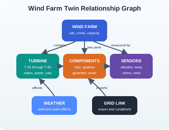
What relationships would you model in your twin graph?
How would you handle a turbine going offline for 6 hours?
What predictive analytics would you prioritize?
Solution:
1. Data Ingestion Rate:
- 50 turbines x 100 sensors x 1 reading/second = 5,000 readings/second
- At ~200 bytes per reading: 1 MB/second = 86.4 GB/day raw data
- Architecture: Edge gateway at each turbine for local aggregation, sending only anomalies and 1-minute averages to cloud (99% data reduction). High-frequency raw data stored locally for 48 hours for deep diagnostics on demand.
2. Relationship Model:
3. Turbine Offline Handling:
- Immediate: Mark twin as “DisconnectedState” with last-known values visible
- During Outage: Use neighboring turbine data + weather station to estimate what offline turbine would be experiencing (wake effects, wind patterns)
- Reconciliation: When turbine reconnects, upload locally-stored detailed logs (edge storage). Cloud twin replays historical data to update predictions and calibrate models.
- Alerting: Distinguish network failure from mechanical failure (check adjacent turbines, attempt ping, review last telemetry for anomalies)
4. Priority Predictive Analytics:
- Blade Damage Prediction (highest value): Vibration pattern analysis detects micro-cracks 4-6 weeks before failure. One prevented blade failure saves $500K+ in emergency repairs and downtime.
- Gearbox Wear: Oil analysis + temperature trends predict bearing failures 2-3 weeks ahead. Allows scheduled maintenance vs. emergency shutdown.
- Power Optimization: ML models find optimal yaw angle and blade pitch for current wind conditions, boosting output 2-5%.
- Wake Effect Management: Coordinate turbine orientations to minimize downwind interference, increasing farm-wide efficiency 8-12%.
You might wonder why a wind turbine needs 100 sensors. Here’s why:
Safety: Vibration sensors on blades detect cracks before catastrophic failure. A blade breaking off could destroy the turbine and endanger workers.
Efficiency: Tiny adjustments to blade angle based on wind sensors can boost power output by 5%. Over 50 turbines for 20 years, that’s millions of dollars.
Maintenance: Temperature sensors in the gearbox detect bearing wear weeks before failure. Replacing a bearing costs $50K and takes a day. Emergency repairs after failure cost $500K and two weeks of downtime.
The digital twin correlates all these sensors to find patterns: “When blade vibration increases 3% AND wind gusts exceed 40 mph AND temperature drops below freezing, blade stress reaches dangerous levels.” That’s impossible for humans to spot manually across 50 turbines.
Sammy the Sensor says: “Imagine you have a toy robot that moves around your room. Now imagine you also have a magic mirror that shows a tiny version of your robot inside it. Every time your real robot turns left, the mirror robot turns left too – instantly!”
Lila the Light Sensor adds: “That mirror is a digital twin! But here’s the cool part – the mirror can also talk back to the real robot. If the mirror figures out the robot is about to bump into a wall, it can send a message saying ‘Hey, turn right!’”
Max the Motion Detector explains: “In the lab below, we build exactly this:
- The real thing is an ESP32 chip with a temperature sensor
- The mirror is code that remembers what the temperature was
- When the temperature gets too hot, the mirror turns on an LED light – it is controlling something in the real world!
It is like having a smart friend who watches the thermometer for you and turns on the fan when it gets too warm.”
Bella the Barometer summarizes: “Digital twins are like having a really smart diary for your things. The diary writes down what happens every 2 seconds. Then it can look at the last 10 entries and guess what will happen next. Pretty clever, right?”
25.9 Visual Reference Gallery
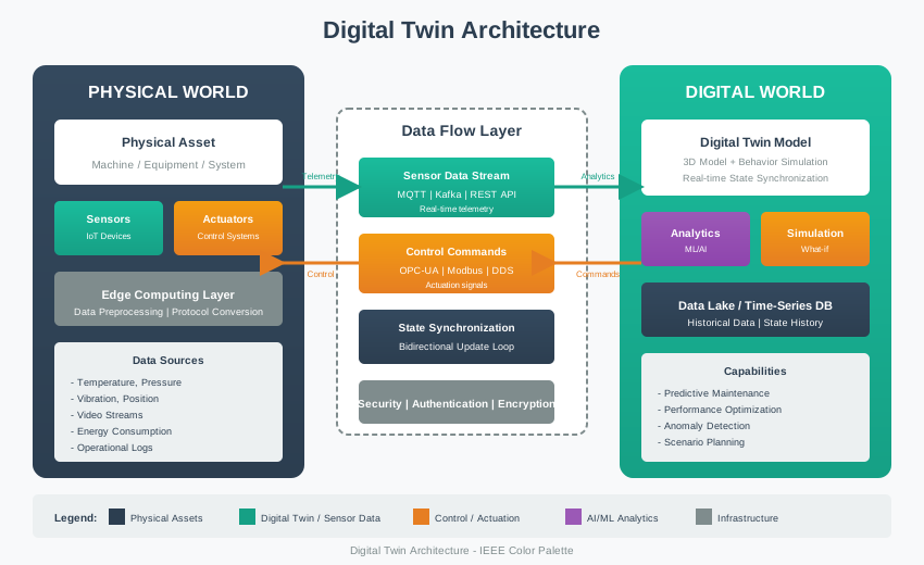
The fundamental architecture of digital twins showing physical-to-virtual synchronization.
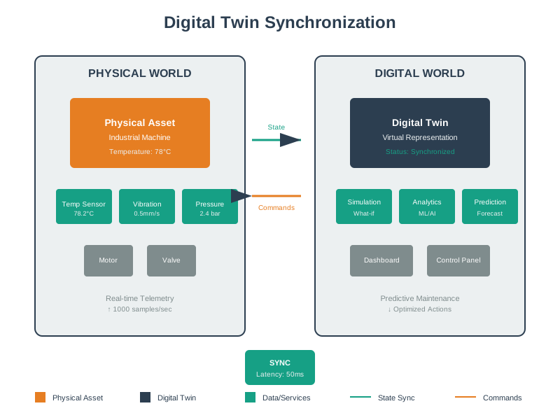
Real-time synchronization between physical systems and their digital counterparts.
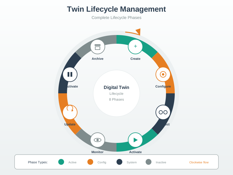
Complete lifecycle management of digital twins from creation to retirement.
25.10 Within This Series
| Direction | Chapter | Topic |
|---|---|---|
| Current | Digital Twin Concepts and Scenario Assessment | Architecture concepts, quizzes, and scenario questions |
| Next | Lab: Build a Digital Twin | Hands-on ESP32 build with sync, history, prediction, and commands |