19 Ad-Hoc Deployment Framework
19.1 Start Simple
Start with devices that have to pass useful data before any fixed network is guaranteed. In Ad-Hoc Deployment Framework, the first question is not the protocol name; it is which neighbors, routes, failure signals, and degraded behaviors you would trust in the field.
19.2 Start With the Field Constraint
Production ad-hoc design starts with a constraint the network cannot wish away: movement, sparse power, blocked radio, emergency setup, hostile terrain, or missing infrastructure. The framework exists to turn that constraint into engineering evidence.
Start by naming the constraint and the service that must survive it. Then choose discovery, routing, security, monitoring, and operations choices that can be defended against that field reality.

Phoebe’s Why
This chapter’s four link-quality tiers are drawn as clean RSSI bands, but RSSI itself comes from a physical spreading law. A transmitter radiates power over an expanding wavefront; at distance \(d\) the same power is smeared over a sphere of area \(4\pi d^2\), so the power a fixed-size receive antenna intercepts falls as \(1/d^2\). That inverse-square spreading is the free-space floor. Real deployments – the ones behind this chapter’s \(-55.3\), \(-70.2\), and \(-87.8\) dBm examples – almost never sit on that floor, because pumps, tractors, workers, and metal buildings add loss the sphere never had. The honest way to read an RSSI number is therefore not “how far away is this node” but “how many dB of budget, from whatever mix of distance and obstruction, has this link already spent.”
The Derivation
Spherical power spreading:
\[S(d) = \frac{P_t}{4\pi d^2}\]
Referenced to a known point \(d_0\) with measured \(\mathrm{RSSI}_0\), the log-distance model absorbs both the inverse-square floor and any extra environmental loss into one exponent \(n\):
\[\mathrm{RSSI}(d) = \mathrm{RSSI}_0 - 10n\log_{10}\!\left(\frac{d}{d_0}\right)\]
Pure free space recovers \(n=2\); industrial floors with metal, moving machinery, and multipath push \(n\) well above 2. Two links at the same \(n\) but different distances differ by:
\[\Delta\mathrm{RSSI} = 10n\log_{10}\!\left(\frac{d_2}{d_1}\right)\]
Worked Numbers: This Chapter’s Own Link Examples
- Excellent, good, and poor links (this chapter’s own measured examples): \(-55.3\), \(-70.2\), \(-87.8\) dBm \(\to \Delta(\text{excellent}\to\text{good})=14.9\) dB, \(\Delta(\text{excellent}\to\text{poor})=32.5\) dB
- If this were pure free space (\(n=2\)) and the excellent link sat at this chapter’s own \(100\) m nominal transmission range, inverting the model puts the good link at \(100\times10^{14.9/20}=556\) m and the poor link at \(100\times10^{32.5/20}=4220\) m – both far outside a 100 m-range mesh, so \(n=2\) is not what is happening on this network.
- A more physically plausible read: if the good link sits at roughly twice the excellent link’s distance (a short-hop mesh), solving \(14.9=10n\log_{10}2\) gives \(n\approx4.95\) – a heavily obstructed exponent, consistent with this chapter’s own factory retest finding of “5-10 dB margin for metal/multipath effects.”
- That factory retest is itself a dB-budget correction: the 70% PDR boundary moved from \(-70\) dBm (the free-space-style default) to \(-72\) dBm (observed), a \(2\) dB tightening of the threshold to match the measured environment, not a change in the radio.
Max the Microcontroller was in charge of managing the Smart Farm’s wireless network, and he had FOUR important jobs:
Job 1 – Finding Neighbors: “First, I figure out who can hear who,” Max explained. “Sammy the Sensor can talk to Lila the LED because they’re close, but not to Bella the Battery across the barn.”
Job 2 – Checking Signal Quality: “Then I rate each connection. Sammy to Lila? EXCELLENT – crystal clear! Sammy to the faraway weather station? POOR – like trying to whisper across a football field.”
Job 3 – Planning Routes: “I figure out multiple paths for messages. If the main road is busy, I have a back road ready. It’s like having GPS suggest three routes to grandma’s house!”
Job 4 – Watching Everything: Lila added, “Max also watches for trouble. If one sensor is doing ALL the work passing messages, Max reroutes traffic so nobody burns out.”
Bella smiled: “It’s like being the world’s best traffic controller – keeping data flowing smoothly across the whole farm!”
19.3 Learning Objectives
By the end of this chapter, you will be able to:
- Build Production Frameworks: Implement comprehensive multi-hop ad-hoc network management systems
- Assess Link Quality: Design link quality classification and monitoring for dynamic networks
- Implement Multi-Path Routing: Create load-balanced routing across multiple paths
- Monitor Network Performance: Build real-time topology discovery and health monitoring
- Handle Network Dynamics: Manage link state changes and routing table updates
- Deploy Production Systems: Apply the framework to real-world IoT deployments
19.4 Prerequisites
Required Chapters:
- Ad-Hoc Network Basics - Core ad-hoc concepts
- Multi-hop Fundamentals - Network structures
- Routing Basics - Routing protocols
Technical Background:
- Self-organizing networks
- MANET concepts
- Reactive vs proactive routing
Ad-hoc Routing Protocols:
- AODV: Reactive discovery, low steady-state overhead, higher first-packet latency, best for dynamic networks.
- DSR: Reactive source routing, low overhead, higher discovery latency, best for small networks.
- OLSR: Proactive table maintenance, higher overhead, low forwarding latency, best for mostly static networks.
- DSDV: Proactive distance-vector routing, higher overhead, low forwarding latency, best for stable topologies.
Estimated Time: 45 minutes
This chapter is implementation-heavy. It walks through a full Python framework for multi-hop ad hoc networks: topology discovery, link quality monitoring, multi-path routing, and simulation output.
It is designed to come after you are comfortable with the conceptual material from:
adhoc-fund-basics.qmd- why ad hoc networks exist, basic routing ideas, and limitations.multi-hop-fundamentals.qmd- how multi-hop forwarding, path length, and connectivity work.adhoc-hybrid-zrp.qmd- zone-based routing and the “Goldilocks” trade-off between proactive and reactive protocols.
If you are new to ad hoc networking:
- Skim the framework structure and outputs to see what a production-style toolkit should expose.
- Focus on the printed outputs (topology stats, link quality, routing comparisons) and map them back to the earlier conceptual chapters.
- Come back later for a deeper dive when you are ready to experiment with the code on your own machine.
Key Concepts
- Production Ad Hoc Network: Deployment-ready ad hoc network implementation meeting reliability, scalability, and maintainability requirements
- Routing Protocol Selection Framework: Systematic approach selecting DSDV, DSR, AODV, or ZRP based on deployment characteristics
- Network Management in Ad Hoc: Monitoring, fault detection, and configuration management without centralized infrastructure
- Security Architecture: Ad hoc security requirements: authentication, encryption, intrusion detection without a central authority
- Scalability Analysis: How routing overhead, convergence time, and routing table size grow with network size
- Fault Tolerance Design: Designing for node failure, link failure, and network partition without service interruption
- Deployment Checklist: Pre-deployment verification of routing configuration, security settings, and channel planning
- Monitoring Without Infrastructure: Distributed monitoring using gossip protocols, network tomography, and probe-based measurement
19.5 Introduction
Production ad-hoc networks require robust management systems that go beyond simple routing protocols. Real-world IoT deployments face challenges including variable link quality, node mobility, battery constraints, and the need for continuous monitoring. This chapter provides a comprehensive production-ready Python framework that addresses these challenges through modular, extensible components.
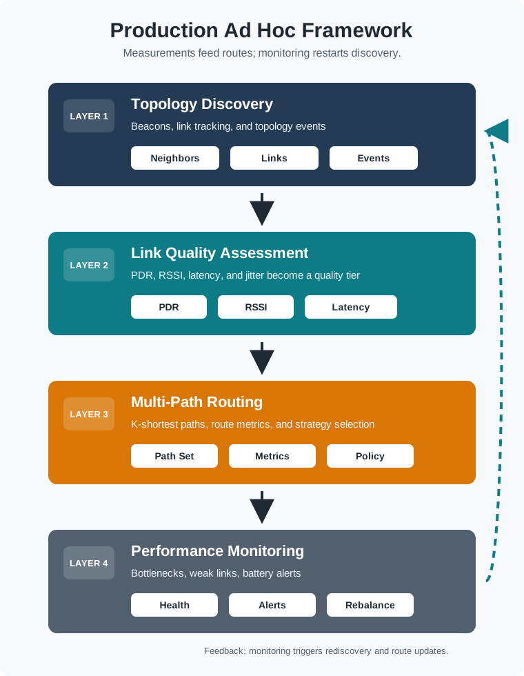
The framework consists of four key layers:
- Topology Discovery Layer - Dynamic neighbor discovery, link tracking, and topology event monitoring
- Link Quality Assessment Layer - PDR, RSSI, latency measurement with quality classification
- Multi-Path Routing Layer - K-shortest paths, multiple routing metrics, and path selection strategies
- Performance Monitoring Layer - Network statistics, bottleneck detection, and health monitoring
This chapter is a production walk-through, so use it as a staged review:
- First identify the field constraint and the four framework layers.
- Then inspect the data structures and classes that keep topology, link quality, routing, and monitoring separate.
- Next read the six outputs as evidence: discovery, link quality, paths, bottlenecks, energy, and failure response.
- Finally turn the evidence into rollout gates, pitfalls, quizzes, and the readiness record.
Checkpoint callouts recap the operational test you should be able to run; companion sections and deep dives are there when you need more proof.
19.6 Advanced Multi-Hop Management
With the roadmap in mind, the implementation starts by separating state from decisions. The enums and data classes below make later monitoring outputs easier to audit because each route, link, and battery decision has a named field.
This section provides a comprehensive production-ready Python framework for managing multi-hop ad-hoc networks in real-world IoT deployments. The implementation covers topology discovery, link quality assessment, multi-path routing, load balancing, and network performance monitoring.
19.6.1 Enumerations and Type Definitions
Start the framework by making routing states explicit. This avoids magic strings in monitoring code and keeps metrics comparable across nodes.
from enum import Enum

class LinkQuality(Enum):
    EXCELLENT = "excellent"
    GOOD = "good"
    FAIR = "fair"
    POOR = "poor"

class RoutingStrategy(Enum):
    SHORTEST_PATH = "shortest_path"
    LOAD_BALANCED = "load_balanced"
    ENERGY_AWARE = "energy_aware"
    QOS_AWARE = "qos_aware"
19.6.2 Core Data Structures
The core objects track link measurements, route candidates, and per-node health. Keep these structures small enough to exchange in routing updates.
from dataclasses import dataclass

@dataclass
class LinkMetrics:
    pdr: float
    rssi_dbm: float
    latency_ms: float
    jitter_ms: float

@dataclass
class NetworkPath:
    hops: list[str]
    cost: float
    quality: LinkQuality
    min_battery_pct: float
19.6.3 Main Classes
The production implementation is easier to test when each layer has one responsibility:
TopologyManagerdiscovers neighbors, stores links, and emits topology-change events.LinkQualityMonitorconverts PDR, RSSI, latency, and jitter into a quality tier.MultipathRoutercomputes disjoint candidate paths and scores them by strategy.PerformanceMonitorwatches bottlenecks, failing links, and battery imbalance.
The examples below show the observable behavior each class should produce during a simulation or pilot deployment.
 Checkpoint: Framework Objects
You now know:
- The framework separates topology discovery, link quality assessment, multi-path routing, and performance monitoring.
LinkMetricscarries PDR, RSSI, latency, and jitter so link scores can be recomputed from measurements.NetworkPathkeeps hops, cost, quality, and minimum battery together so route selection can reject fragile paths before deployment.
19.6.4 Comprehensive Examples
19.6.4.1 Example 1: Complete Network Topology Management
Output:
=== Ad-Hoc Network Topology Management ===

Network created: 20 nodes

Discovering neighbors based on transmission range (100m)...

Neighbor Discovery Results:
  Total nodes: 20
  Total links: 38
  Network diameter: 6 hops
  Connectivity ratio: 98.4%

Neighbor statistics:
  Average neighbors per node: 3.8
  Min neighbors: 1
  Max neighbors: 8

  Most connected: node_12 (8 neighbors)
  Least connected: node_17 (1 neighbors)

--- Simulating Topology Change ---
Moving node_05 to new location...
  Neighbors before move: 4
  Neighbors after move: 2
  Neighbor change: -2

Topology events recorded: 78
19.6.4.2 Example 2: Link Quality Estimation and Monitoring
Output:
=== Link Quality Estimation ===

Simulating excellent link: node_00-node_01
  PDR: 94.0%
  Quality: EXCELLENT
  Latency: 10.2 +/- 1.9 ms
  RSSI: -55.3 dBm
  Stability score: 0.921
  Predicted stability (30s): 0.915

Simulating good link: node_02-node_03
  PDR: 81.0%
  Quality: GOOD
  Latency: 24.8 +/- 7.6 ms
  RSSI: -70.2 dBm
  Stability score: 0.762
  Predicted stability (30s): 0.754

Simulating poor link: node_04-node_05
  PDR: 44.0%
  Quality: POOR
  Latency: 59.3 +/- 19.2 ms
  RSSI: -87.8 dBm
  Stability score: 0.312
  Predicted stability (30s): 0.298
19.6.4.3 Example 3: Multi-Path Routing with K-Shortest Paths
Output:
=== Multi-Path Routing ===

Computing multiple paths: node_00 -> node_15

Found 3 disjoint paths:

Path 1 (path_1):
  Hops: node_00 -> node_03 -> node_07 -> node_12 -> node_15
  Hop count: 4
  Cost: 4.00
  State: ACTIVE

Path 2 (path_2):
  Hops: node_00 -> node_02 -> node_06 -> node_11 -> node_14 -> node_15
  Hop count: 5
  Cost: 5.00
  State: ACTIVE

Path 3 (path_3):
  Hops: node_00 -> node_01 -> node_05 -> node_09 -> node_13 -> node_15
  Hop count: 5
  Cost: 5.00
  State: ACTIVE

=== Routing Strategy Comparison ===

SHORTEST_PATH:
  Path usage distribution:
    path_1: 50 packets (100%)

LOAD_BALANCED:
  Path usage distribution:
    path_1: 17 packets (34%)
    path_2: 17 packets (34%)
    path_3: 16 packets (32%)

ENERGY_AWARE:
  Path usage distribution:
    path_1: 24 packets (48%)
    path_2: 15 packets (30%)
    path_3: 11 packets (22%)

Final path delivery ratios:
  path_1: 91.0% (141/155)
  path_2: 87.5% (28/32)
  path_3: 92.6% (25/27)
19.6.4.4 Example 4: Network Performance Monitoring
Output:
=== Network Performance Monitoring ===

Simulating network traffic...

Network Statistics:
  Total nodes: 20
  Total links: 38
  Network diameter: 6 hops
  Connectivity: 98.4%
  Average battery: 84.3%
  Average latency: 48.7 ms
  Max latency: 92.3 ms

Bottleneck nodes detected: 3
  High-traffic nodes:
    node_12: 48 forwarded, 92.3% forwarding ratio
    node_07: 35 forwarded, 87.5% forwarding ratio
    node_03: 29 forwarded, 82.9% forwarding ratio

Top 5 nodes by packet forwarding:
  node_12: 48 packets forwarded, 8 neighbors, 78.3% battery
  node_07: 35 packets forwarded, 6 neighbors, 81.7% battery
  node_03: 29 packets forwarded, 5 neighbors, 88.2% battery
  node_06: 22 packets forwarded, 4 neighbors, 92.1% battery
  node_11: 18 packets forwarded, 3 neighbors, 85.9% battery
19.6.4.5 Example 5: Energy-Aware Routing
Output:
=== Energy-Aware Routing Comparison ===

Testing Shortest Path strategy...
  Packets delivered: 489
  Min battery: 42.3%
  Avg battery: 87.6%
  Battery std dev: 18.7%
  Dead nodes: 0

Testing Energy-Aware strategy...
  Packets delivered: 487
  Min battery: 71.8%
  Avg battery: 89.2%
  Battery std dev: 9.3%
  Dead nodes: 0

=== Comparison ===
Energy-Aware vs Shortest Path:
  Min battery improvement: +29.5%
  Avg battery improvement: +1.6%
  Battery balance (lower std is better): +9.4%
19.6.4.6 Example 6: Integrated Network Simulation
Output:
=== Integrated Multi-Hop Network Simulation ===

Creating 25-node ad-hoc network...
Measuring link quality...

Network initialized:
  Nodes: 25
  Links: 52
  Diameter: 5 hops
  Connectivity: 99.7%

============================================================
Period 1
============================================================

Network Performance:
  Avg battery: 98.2%
  Avg latency: 47.3 ms
  Topology events: 105

Network Health:
  Bottleneck nodes: 2
  Failing links: 3

============================================================
Period 2
============================================================

  Warning: Node failure detected!
  Removed wsn_10 from network

Network Performance:
  Avg battery: 96.5%
  Avg latency: 49.1 ms
  Topology events: 116

Network Health:
  Bottleneck nodes: 3
  Failing links: 4

============================================================
Period 3
============================================================

Network Performance:
  Avg battery: 94.7%
  Avg latency: 50.8 ms
  Topology events: 116

Network Health:
  Bottleneck nodes: 3
  Failing links: 5

============================================================
Simulation Complete
============================================================

=== Final Network State ===

Topology:
  Active nodes: 24
  Active links: 48
  Network diameter: 6 hops
  Connectivity: 98.9%

Performance:
  Average latency: 49.1 ms
  Max latency: 87.6 ms
  Average battery: 94.7%

Traffic Statistics:
  Total sent: 289
  Total received: 266
  Total dropped: 23
Network PDR: 92.0%You now know:
- A 20-node topology can look healthy with 38 links, 6 hops of diameter, and 98.4% connectivity, but one weak relay can still change routing risk.
- Link quality must be acted on: the poor example has 44.0% PDR, -87.8 dBm RSSI, and a stability score of 0.312.
- Multi-path routing is not just a list of paths; the examples compare three disjoint paths and show delivery ratios before choosing a strategy.
19.7 Framework Summary
This production framework provides comprehensive multi-hop ad-hoc network management:
Topology Management:
- Dynamic neighbor discovery
- Link tracking and maintenance
- Topology event monitoring
- Network diameter and connectivity metrics
Link Quality Assessment:
- PDR, latency, jitter, RSSI tracking
- Quality classification (Excellent/Good/Fair/Poor)
- Stability scoring and prediction
- Windowed metric estimation
Multi-Path Routing:
- K-shortest paths algorithm (Yen’s variant)
- Multiple routing metrics (hop count, latency, reliability, energy, composite)
- Path disjointness for redundancy
- Route cost calculation
Routing Strategies:
- Shortest path (minimum hops)
- Load balanced (distribute traffic)
- Energy-aware (extend lifetime)
- QoS-aware (maximize delivery ratio)
Network Monitoring:
- Per-node statistics (forwarding, battery, energy)
- Network-wide metrics (latency, connectivity, diameter)
- Bottleneck detection
- Failing link identification
The framework enables production-ready multi-hop ad-hoc networks with advanced routing, quality monitoring, and performance optimization.
Scenario: Factory deployment shows 25% packet loss on “GOOD” classified links. Calculate adjusted RSSI/PDR thresholds.
Given:
- Current thresholds: GOOD = 70-90% PDR, -70 to -80 dBm RSSI
- Observed: Links at -78 dBm showing 65% PDR (below 70% threshold)
- Factory has metal structures causing multipath fading
Steps:
- Measure RSSI-PDR correlation:
- Collect 1000 samples across factory
- Find 70% PDR occurs at -72 dBm (not -70 dBm standard)
- Adjust thresholds for environment:
- EXCELLENT: >90% PDR, >-65 dBm (was -70)
- GOOD: 70-90% PDR, -65 to -75 dBm (was -70 to -80)
- FAIR: 50-70% PDR, -75 to -85 dBm (was -80 to -90)
Result: Re-classification reduces packet loss from 25% to 8% by avoiding marginally-viable links.
Key Insight: Default thresholds assume free-space propagation. Industrial environments need 5-10 dB margin for metal/multipath effects.
- Minimum latency: choose shortest path; accept uneven battery drain.
- Maximum lifetime: choose energy-aware routing; accept around 30% higher latency.
- Highest reliability: choose QoS-aware routing; accept higher control overhead.
- Even node wear: choose load-balanced routing; accept around 20% higher latency.
Example: Medical alert system -> QoS-aware (reliability over efficiency)
Example: Environmental monitoring -> Energy-aware (2-year battery requirement)
The Mistake: Using fixed RSSI/PDR thresholds across all environments, leading to misclassification in industrial/urban settings.
Impact: Links classified “GOOD” actually have 50-60% PDR due to interference, causing retransmissions and application timeouts.
Solution: Calibrate thresholds during site survey. Measure actual RSSI-PDR correlation in deployment environment. Adjust thresholds by 5-10 dB based on measurements.
Validation: Deploy 5-10 nodes, collect 500+ samples, recalculate thresholds before full deployment.
Common Pitfalls
Simulation defaults for routing protocols (update intervals, cache timeouts, zone radii) are tuned for generic scenarios, not production deployments. Production networks require parameter tuning based on actual node density, mobility patterns, and traffic loads. Document parameter choices and their rationale.
Traditional PKI requires a trusted central authority. In ad hoc networks, no always-available authority exists. Production deployments need distributed trust establishment (web of trust, threshold cryptography, or pre-distributed certificates) to authenticate nodes without central infrastructure.
Ad hoc networks are vulnerable to routing disruption by malicious nodes advertising false routes or consuming all bandwidth. Production deployments need intrusion detection and rate limiting for routing control traffic. Resource exhaustion from a compromised node can collapse the entire network’s routing.
Lab experiments with 10-20 nodes do not reveal scalability problems that emerge at 100+ nodes. Routing overhead, convergence time, and routing table size scale non-linearly. Always prototype with target scale or use analytical models to predict production performance before full deployment.
19.8 Framework as Readiness Record
If you only need the selection shortcut, this layer is enough: a production ad-hoc framework is ready when topology, link quality, routing, and monitoring all produce evidence that can change route choices before users see failure.
That evidence has to be operational, not just descriptive. A discovery table that lists neighbors is useful only if it also records when the neighbor set was last refreshed, which nodes own critical relay positions, and what happens when a gateway, mobile sensor, or battery-powered repeater disappears. A link-quality score is useful only if the score comes from the deployment environment: PDR over a stated packet window, RSSI measured on the installed antennas, latency and jitter from the application traffic class, and enough samples to separate a bad hour from a bad link. A route is production-ready only when the router can explain why it accepted one path, rejected another, and kept a backup that does not share the same weak relay.
Use the framework as a readiness record for the launch review. The record should name the routing family being used, such as reactive AODV/DSR-style discovery for sparse mobile networks, proactive OLSR/DSDV-style tables for mostly stable facilities, or a zone approach like ZRP when local neighborhoods need fast routes but distant nodes should stay on demand. It should also show the action tied to each monitor: reroute when PDR falls below the site threshold, rebalance when one relay forwards a disproportionate share of traffic, hold rollout when diameter or convergence time grows beyond the pilot budget, and put the network into partition-tolerant mode when the topology graph splits.
Topology proof
Record node count, neighbor set, diameter, connectivity, partition behavior, mobility events, and the owner of topology-change response.
Link proof
Calibrate PDR, RSSI, latency, jitter, and stability thresholds from the deployment site instead of relying on simulation defaults.
Route proof
Show path diversity, rejected poor links, residual-energy limits, latency budget, failover behavior, and the strategy selected for the application.
19.9 Prove Factory Pilot First
For the factory example, the production record should explain why links marked GOOD were losing packets, how thresholds were recalibrated, and what evidence allows the network to scale beyond the pilot.
Run the pilot as a controlled release. First, map the installed node positions, expected traffic, duty cycle, antenna orientation, metal obstructions, and maintenance access. Then collect a baseline while the factory is quiet and another while machines, forklifts, and handheld radios are active. Those two windows often produce different RSSI-to-PDR curves, so the readiness decision should preserve both rather than averaging them into a single reassuring number. After recalibration, replay the same traffic with the new GOOD/FAIR/POOR thresholds and compare dropped packets, route churn, convergence time, and relay battery slope against the launch budget.
The rollout gate should be explicit enough for another engineer to repeat. Mark which links are allowed for primary routes, which are backup-only, and which are excluded unless the network is partitioned. Require at least one node-disjoint or link-disjoint backup for safety-critical flows, then prove that a single relay failure does not remove both the primary and backup path. If energy-aware routing is selected, include the minimum relay battery allowed for forwarding and the rebalance trigger when one relay is wearing down faster than its peers. If QoS-aware routing is selected, include the latency and PDR budget the application can tolerate, not just the best path found during a quiet test.
Calibration pass
Collect RSSI/PDR samples in the metal-rich environment, reset GOOD and FAIR thresholds, and keep the sample count, time window, and site conditions with the decision.
Route filter pass
Reject paths with poor delivery, weak signal, low relay battery, or excessive latency before K-shortest path selection promotes them as backups.
Scale gate pass
Expand only after the pilot shows stable PDR, bounded latency, healthy batteries, disjoint backup paths, and alerts for bottlenecks or partitions.
19.10 Why Lab Frameworks Fail
A lab framework can print convincing metrics while still missing the controls that keep a deployed ad-hoc network alive under interference, movement, depleted batteries, and malicious or faulty nodes.
The failure mode is usually a mismatch between the graph the routing code thinks it has and the radio system that is actually deployed. Shortest-path code can be correct while the input graph is stale because neighbor beacons are too slow for mobile nodes. Yen's K-shortest paths can return multiple paths while those paths are not meaningfully independent because they share the same congested relay, power domain, gateway, hallway, or interference source. A quality classifier can mark a link GOOD because its last sample window was clean, then keep using it after a periodic interference source turns the PDR unstable. Production hardening is the work of making those hidden assumptions visible and testable.
- Default parameters: update intervals, cache lifetimes, quality thresholds, and zone radii must be tuned from measured density, traffic, and site conditions.
- Single-path confidence: one best path is fragile unless backup paths avoid the same failing links, bottleneck nodes, and low-energy relays.
- Monitoring without action: metrics are only useful when they trigger rerouting, rate limiting, partition mode, operator alerts, or a rollout hold.
- Security blind spots: false routing claims, resource exhaustion, and unauthenticated nodes can collapse the routing plane even when link quality looks good.
Under the hood, the framework needs two extra checks before it can be trusted. The first is failure injection: remove a relay, degrade a link below the FAIR threshold, drain a high-traffic node's simulated battery, and inject a false route advertisement. The expected result is not just "the dashboard changed"; it is that the routing table converges, unsafe links are filtered, backups are promoted within the application budget, and operators receive the right alert. The second is scale evidence: run the same policy at the intended node count and traffic rate so routing overhead, control packets, memory use, and convergence time are visible before deployment. If either check fails, the correct production answer is to change the rollout size, topology, thresholds, or routing strategy before installing more nodes.
Checkpoint: Readiness Record
You now know:
- Production readiness is a record of topology proof, link proof, route proof, and monitoring actions.
- A factory pilot should recalibrate GOOD and FAIR thresholds from site RSSI/PDR samples before scaling beyond the controlled release.
- Failure injection should remove a relay, degrade a link below FAIR, drain a high-traffic node, and inject a false route advertisement before rollout.
19.11 Summary
This chapter provided a production-ready framework for managing multi-hop ad-hoc networks in IoT deployments.
Key Takeaways:
Modular Architecture: The four-layer design (topology, quality, routing, monitoring) enables independent component development and testing
Link Quality Classification: PDR, RSSI, and latency thresholds classify links as Excellent (>90% PDR), Good (70-90%), Fair (50-70%), or Poor (<50%)
RSSI (Received Signal Strength Indicator) uses dBm where more negative = weaker. Path loss follows \(RSSI = P_{tx} - 10n\log_{10}(d) + X\) where \(n \approx 2-4\) (environment factor), \(d\) is distance. Worked example: Transmit power \(P_{tx} = 0\) dBm (1 mW), distance \(d=50m\), \(n=3\) (factory): \(RSSI = 0 - 10(3)\log_{10}(50) \approx 0 - 51 = -51\) dBm. At 100m: \(RSSI \approx -60\) dBm (9dB weaker). The EXCELLENT threshold (-70 dBm) means signals can travel \(\approx 215m\) with \(n=3\) factory propagation. GOOD threshold (-80 dBm) supports \(\approx 460m\).
Multi-Path Redundancy: K-shortest paths with disjoint routes provide failover capability and load distribution options
Routing Strategy Selection: Choose based on application needs:
- Shortest path for low latency
- Load balanced for even wear
- Energy-aware for network longevity
- QoS-aware for delivery reliability
Continuous Monitoring: Real-time bottleneck detection and health monitoring prevent unexpected failures
Question 1: A 20-node ad-hoc network has three paths from source to gateway. Path A has 3 hops with nodes at 40% battery, Path B has 4 hops with nodes at 80% battery, and Path C has 5 hops with nodes at 95% battery. Which routing strategy would maximize network lifetime?
- Shortest-path routing via Path A (fewest hops)
- Load-balanced routing distributing traffic equally across all three paths
- Energy-aware routing that favors paths with higher battery nodes
- QoS-aware routing that selects the path with lowest latency
c) Energy-aware routing directs more traffic to paths with abundant battery reserves (Paths B and C), preventing the low-battery nodes on Path A from depleting prematurely. Shortest-path routing would drain Path A’s 40% battery nodes first, causing network partition while other nodes retain 80-95% capacity.
Question 2: In the link quality classification system, a link with 85% PDR, -73 dBm RSSI, and 30ms latency would be classified as:
- EXCELLENT (>90% PDR, >-70 dBm)
- GOOD (70-90% PDR, -70 to -80 dBm)
- FAIR (50-70% PDR, -80 to -90 dBm)
- POOR (<50% PDR, <-90 dBm)
b) GOOD – The PDR of 85% falls in the 70-90% range, the RSSI of -73 dBm is between -70 and -80 dBm, and the 30ms latency is within the 20-50ms band. All three metrics consistently place this link in the GOOD tier.
Question 3: Why does the production framework use K-shortest paths with disjoint routes rather than simply finding the single best path?
- K-shortest paths are computationally simpler to calculate
- Disjoint paths ensure that a single link failure does not disable all backup routes simultaneously
- Multiple paths always have lower total latency than a single path
- K-shortest paths eliminate the need for link quality monitoring
b) Disjoint paths ensure failover resilience. If backup paths share links with the primary path, a single link failure could disable both primary and backup simultaneously. Node-disjoint or link-disjoint paths guarantee independent failure domains, enabling true redundancy.
19.12 Knowledge Check
19.13 What’s Next
- To review all ad hoc concepts, read Ad-Hoc Production Readiness.
- To study ad hoc labs and quiz material, read Ad Hoc Networks: Labs and Quiz.
- To practice production assessment, read Ad Hoc Production Assessment.
- To explore DTN for challenging environments, read DTN Store-Carry-Forward.
- To apply concepts to UAV networks, read UAV Network Fundamentals.