12 DTN Store-Carry-Forward
emerging-paradigms
adhoc
dtn
12.1 Start Simple
Start with devices that have to pass useful data before any fixed network is guaranteed. In DTN Store-Carry-Forward, the first question is not the protocol name; it is which neighbors, routes, failure signals, and degraded behaviors you would trust in the field.
12.2 Start With a Network That Is Usually Broken
A delay-tolerant network assumes that end-to-end connectivity may not exist when a message is created. A node stores data, carries it through time and space, and forwards it when contact finally appears.
That idea fits wildlife sensors, rural links, disaster response, ships, vehicles, and remote field work. Start with one message that cannot be delivered now. The DTN story is how the system protects it until delivery becomes possible.
Chapter Roadmap
Read this chapter as a sequence of field decisions:
- First decide whether the network is actually disconnected, rather than merely slow.
- Then build a delivery record for one bundle class: payload, destination, deadline, priority, contact assumptions, buffer limit, custody rule, and failure action.
- Next compare ordinary ad hoc routing with DTN store-carry-forward, using wildlife, rural kiosk, disaster, and space examples.
- Finally run the elephant tracking numbers through buffer, contact, latency, energy, and delivery reliability before choosing a copy policy.
Checkpoints recap what you have covered; the audit panel supports number verification.
Sensor Squad: The Traveling Mailbox
“Oh no!” cried Sammy the Sensor. “I need to send my temperature reading to the base station, but it’s 10 kilometers away and my radio only reaches 100 meters!”
Bella the Battery shook her head. “There’s no Wi-Fi tower, no phone tower, nothing in between. Traditional networking says: ‘Sorry, network unreachable!’”
“But wait!” said Max the Microcontroller. “What if a friendly delivery truck drives by tomorrow? Sammy could hand the message to the truck driver, the driver carries it across the desert, and drops it off at the base station!”
“That’s Store-Carry-Forward!” Lila the LED explained. “Store the message in memory, Carry it while you move, Forward it when you meet someone heading the right way. It might take a day instead of a second, but the message GETS THERE!”
Real-world example: In Africa, zebras wear GPS collars. When two zebras meet at a watering hole, their collars swap data. Days later, one zebra wanders near a base station and all the data downloads. Scientists get their migration maps – just a few days late!
12.3 Learning Objectives
By the end of this chapter, you will be able to:
- Explain DTN Concepts: Describe Delay-Tolerant Networks and their fundamental assumptions about disconnection
- Analyze Disconnected Scenarios: Identify IoT applications where continuous connectivity is unavailable and justify DTN suitability
- Apply Store-Carry-Forward: Implement the core DTN paradigm for intermittent connectivity in real deployments
- Distinguish DTN from Traditional Routing: Compare DTN approaches with connected ad hoc protocols and evaluate when each is appropriate
12.4 Disconnection Comes First
If you only need the intuition, this layer is enough: DTN works when a packet cannot follow a continuous path. A node stores the bundle, carries it while moving, and forwards it during a later contact.
That changes the design question. In a connected IP network, the first question is often "which next hop can carry this packet now?" In a DTN, the first question is "what state must survive until a useful contact appears?" The message needs an identity, a destination, a creation time, an expiration rule, and enough priority context for a future carrier to decide whether it deserves buffer space.
A good mental model is a traceable handoff chain. A sensor may create a bundle at noon, a vehicle may collect it at sunset, another gateway may receive it the next morning, and the application may still accept it because the measurement is late but useful. The same design is wrong when the data loses value in seconds, when storage cannot survive the gap, or when the operator cannot explain what happens after a missed contact.
This is why DTN chapters should talk about time as a normal part of routing. The path is not just a set of radios; it is a sequence of storage intervals and contact opportunities. A store-carry-forward design is ready to discuss only when the team can name the expected delay range and the application consequence of arriving outside it.
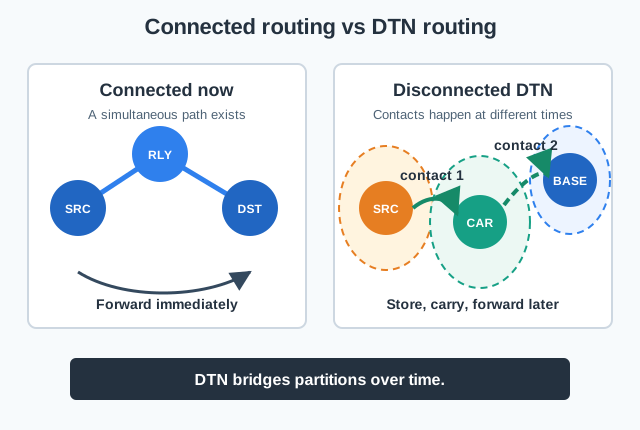
Mobile summary: connected ad hoc routing needs a simultaneous path, while DTN assumes the path is broken and uses storage plus movement to bridge contacts over time.
Store
The source writes the bundle to persistent storage instead of dropping it when no route exists.
Carry
A person, animal, vehicle, drone, or satellite physically moves the stored bundle through the disconnected region.
Forward
The carrier transfers the bundle when a useful contact appears and the receiving node can take responsibility.
 Checkpoint: Disconnection Frame
You now know:
- DTN starts from the assumption that no simultaneous end-to-end path may exist.
- Store-carry-forward turns storage intervals, mobility, and later contact windows into the path.
- The first design question is what state must survive until contact appears.
12.5 Practitioner: Build the Delivery Record
A DTN design should start with one bundle class and a delivery promise. Wildlife GPS summaries, disaster status reports, and rural kiosk messages can tolerate delay, but each still needs a record that proves the delay is acceptable and bounded.
The delivery record should be concrete enough for a field review. Name the bundle identifier scheme, payload size range, producer, destination endpoint, maximum useful age, priority, privacy sensitivity, and duplicate-handling rule. Then name the storage owner at each stage: source node, mobile carrier, relay cache, gateway, or application server. If ownership is vague, stale bundles tend to accumulate because every device assumes another device is responsible for cleanup.
Contact evidence turns the design from a story into an engineering budget. For example, a 20-second contact at 50 kbit/s can move at most about 125 kB before protocol overhead, retries, and radio setup time. If the daily payload is larger than the contact budget, the design needs compression, prioritization, more contacts, a higher-rate link, or a decision to drop low-value bundles. The record should include a replay test for missed contacts, full buffers, duplicate arrivals, and expired data.
Finally, make the record operational. Put the bundle fields, contact assumptions, and failure actions in the same runbook operators use after deployment. When a field technician sees an expired bundle counter rising or a carrier returning with a full buffer, the runbook should say whether to change TTL, reduce sampling, add storage, change the collection route, or escalate the application requirement.
Bundle meaning
Name the payload, producer, destination, deadline, priority, and whether duplicate delivery is acceptable.
Contact evidence
Record expected contacts, radio range, transfer window, data volume, contact rate, and mobility assumption.
Buffer policy
Set storage limits, time-to-live, custody rule, retry rule, and drop order before field deployment.
Failure action
Define what the system does when a bundle expires, custody fails, storage fills, or a planned contact never occurs.
12.6 Buffers Become the Network
In connected routing, a packet mostly lives in transit. In DTN, the packet may spend most of its life inside node storage. That makes buffer management, custody transfer, expiration, and contact prediction first-class network behavior rather than implementation details.
The buffer is not just a cache. It is a queue with durability, ordering, and deletion semantics. The implementation has to survive power loss during a write, keep enough metadata to resume after reboot, and avoid admitting a new bundle that forces out a more valuable one without following the configured drop rule. This is why persistent storage wear, flash capacity, and metadata integrity belong in the network review.
Custody is also a policy boundary, not a magic guarantee. A receiver that accepts responsibility may allow the sender to reclaim storage, but that receiver can still lose power, fill its buffer, miss the next contact, or expire the bundle before delivery. Practical systems therefore keep acknowledgement state, retry limits, and delivery reports separate from the physical act of copying bytes. A copied bundle is not necessarily a delivered bundle.
Contact prediction can be simple or sophisticated, but it must be testable. A bus schedule, a satellite pass table, a patrol route, historical encounter logs, or received-signal observations can all drive forwarding choices. The under-the-hood review should ask what evidence updates that prediction and what the system does when the prediction is wrong. Without that rule, the same bundle may be carried by the wrong node while a better carrier passes nearby.
- Persistent storage: bundles must survive sleep cycles, movement, reboot, and long gaps between contacts.
- Custody transfer: a receiver may take responsibility so the sender can reclaim storage, but custody does not guarantee success.
- Time-to-live: stale bundles should expire before they crowd out higher-priority or fresher messages.
- Contact economics: every contact window has limited time, bandwidth, energy, and competing bundles.
Checkpoint: Delivery Record
You now know:
- A DTN design should start with one bundle class and a delivery promise.
- The record needs bundle meaning, contact evidence, buffer policy, and failure action.
- A 20-second contact at 50 kbit/s moves at most about 125 kB before overhead, retries, and setup time.
12.7 Prerequisites
Before diving into this chapter, you should be familiar with:
- Ad Hoc Routing: Proactive (DSDV): Understanding proactive routing protocols helps contextualize why traditional approaches fail in disconnected networks and how DTN fundamentally differs from table-driven routing
- Ad Hoc Routing: Reactive (DSR): Knowledge of on-demand routing and route discovery mechanisms provides the foundation for understanding why DTN requires store-carry-forward instead of immediate path establishment
- Ad Hoc Routing: Hybrid (ZRP): Zone-based routing concepts introduce the idea of handling disconnected network partitions, which DTN extends with mobility and opportunistic forwarding
- Multi-Hop Fundamentals: Multi-hop networking concepts and relay node behavior are essential background for understanding how DTN leverages mobile nodes as data carriers
- Networking Basics: Fundamental networking concepts, addressing, and packet forwarding provide the baseline understanding for how DTN modifies traditional end-to-end communication
Key Concepts
- DTN (Delay-Tolerant Network): Network architecture accommodating intermittent connectivity, long delays, and high error rates
- Store-Carry-Forward: Core DTN paradigm; nodes store messages locally, carry them as they move, and forward when contact occurs
- Intermittent Connectivity: Characteristic of DTN environments; no end-to-end path exists simultaneously, contacts are opportunistic
- Contact: Period when two DTN nodes can communicate; determined by proximity, mobility patterns, and communication range
- Bundle Protocol: DTN’s network layer (RFC 9171); provides store-and-forward, custody transfer, and end-to-end delivery
- Custody Transfer: DTN mechanism where a receiving node takes responsibility for reliable delivery, allowing the sender to delete its copy
- Disruption Tolerance: DTN’s ability to operate despite network partitions, link failures, and extreme delays (minutes to days)
- Convergence Layer: DTN adaptation layer connecting Bundle Protocol to underlying transport (TCP, Bluetooth, Wi-Fi Direct)
Cross-Hub Connections
Learning Resources:
- Simulations Hub: DTN simulators like The ONE Simulator for testing epidemic routing, spray-and-wait, and social-based protocols in realistic mobility scenarios
- Knowledge Gaps Hub: Common DTN misconceptions including “DTN is just slow networking” and “epidemic routing wastes resources” clarifications
- Videos Hub: Visual explanations of store-carry-forward paradigm, ZebraNet wildlife tracking, and DakNet rural connectivity case studies
- Quizzes Hub: Self-assessment questions on DTN performance trade-offs, utility function design, and protocol selection for intermittent connectivity
Why These Matter:
DTN routing challenges traditional networking assumptions. The Simulations Hub provides hands-on tools to visualize how messages propagate through disconnected networks. Knowledge Gaps addresses the misconception that DTN is simply “broken networking” - it’s actually a deliberate architectural choice for scenarios where continuous connectivity is physically impossible (wildlife tracking, rural areas, disaster zones).
Related Chapters
Deep Dives:
- DTN Epidemic Routing - Flooding-based DTN protocols
- DTN Social Routing - Context-aware and social-based routing
- DTN Applications - Real-world DTN deployments
Protocols:
- Ad Hoc Routing: Proactive (DSDV) - Traditional proactive routing
- Ad Hoc Routing: Reactive (DSR) - Traditional reactive routing
- Ad Hoc Routing: Hybrid (ZRP) - Zone-based routing
- Multi-Hop Fundamentals - Multi-hop communication
Architecture:
- Wireless Sensor Networks - WSN in sparse deployments
- UAV Networks for IoT - Aerial DTN applications
Learning:
- Simulations Hub - DTN simulators
DTN Is Not Just Slow Networking
The Misconception:
Many students think DTN is simply traditional networking with high latency - like a slow internet connection. They assume DTN protocols are inefficient versions of TCP/IP that could be “fixed” with better routing algorithms.
The Reality:
DTN fundamentally differs from traditional networking in its assumptions about connectivity:
Traditional Networks (TCP/IP):
- Assumption: End-to-end path exists when communication starts
- Failure mode: Packets dropped if path breaks during transmission
- Retransmission: Source resends if ACK not received (assumes path will reconnect)
- Use case: Internet, LANs, cellular networks with continuous infrastructure
Delay-Tolerant Networks:
- Assumption: No end-to-end path exists at any single moment
- Acceptance: Disconnection is normal, not a failure condition
- Store-carry-forward: Nodes physically transport data between disconnected regions
- Use case: Wildlife tracking (animals 10km apart), rural areas (no infrastructure), disaster zones (damaged infrastructure)
Concrete Example:
ZebraNet wildlife tracking cannot use traditional TCP/IP because: - Zebras roam 5-20km apart (beyond radio range) - No cellular towers in remote African savanna - Battery budget: 3 years of operation - Data collection: GPS positions every hour
Why TCP/IP fails: Attempting TCP connection from Zebra A to base station fails immediately - no routing path exists. TCP gives up and reports “network unreachable.”
Why DTN works: Zebra A stores GPS data locally. When Zebra B passes within 100m (days later), they exchange buffered data. Zebra B later encounters Zebra C near watering hole base station. Data reaches researchers after 3-7 day delay, which is acceptable for migration studies.
Key Insight:
DTN isn’t “slow networking” - it’s intermittent connectivity networking. Latency isn’t a bug; it’s the price of operation where infrastructure doesn’t exist. The alternative isn’t “faster DTN” - it’s no communication at all.
When to Use:
- No infrastructure possible (wildlife, disaster, space)
- Communication can tolerate hours/days delay
- Mobile nodes can carry data physically
- Real-time requirements (video streaming, gaming)
- Infrastructure available (use Wi-Fi/cellular instead)
We just separated intermittent connectivity from ordinary slow networking. Next, turn that distinction into disconnected ad hoc mechanics: why connected protocols fail, and what replaces them.
12.9 Disconnected Ad Hoc Networks
Traditional routing protocols (DSDV, DSR, ZRP) assume a connected path exists between source and destination. This assumption fails in many IoT scenarios.
12.9.1 Connected vs Disconnected Networks
Disconnected Network Causes:
- Sparse node density: Nodes too far apart for single-connected component
- Node mobility: Moving nodes create temporary islands
- Sleep scheduling: Duty-cycling creates temporal disconnections
- Harsh environment: Obstacles, terrain block connections
- Failure: Node/link failures partition network
Traditional Protocols Fail:
- DSDV: Can’t maintain routes across partitions
- DSR: Route discovery fails if no connected path
- Packets dropped at partition boundaries
12.9.2 Delay-Tolerant Networks (DTN)
Delay-Tolerant Networks enable communication across disconnected networks using store-carry-forward paradigm.
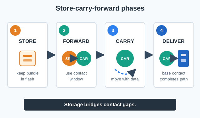
Typical contact sequence:
- The source records data and stores it as a bundle.
- A mobile carrier enters radio range during a contact window.
- The source forwards the bundle to the carrier.
- The carrier physically moves toward another region.
- A later contact with a base station or better relay completes delivery.
DTN Application Scenarios:
- Wildlife tracking: Animals carry sensors, transfer data when near base stations
- Vehicular networks: Cars carry messages between disconnected road segments
- Rural IoT: Mobile collectors (buses, delivery vehicles) gather sensor data
- Disaster recovery: Intermittent connectivity due to infrastructure damage
- Space networks: Planetary exploration with extreme propagation delays
Checkpoint: Store-Carry-Forward Fit
You now know:
- DSDV, DSR, and ZRP assume connected paths; they fail when partitions cannot exchange route messages.
- DTN preserves the bundle locally, carries it on a mobile node, and forwards it during a later contact.
- The correct fit is a delay-tolerant mission: wildlife tracking, vehicular networks, rural IoT, disaster recovery, or space networks.
12.10 DTN Contact Window Calculator
Estimate how much data can be exchanged during an opportunistic DTN contact:
The calculator gives the contact budget. The checks below ask the same question without sliders: can a future contact and local buffer keep the data useful?
12.11 Knowledge Check
Test your understanding of DTN fundamentals.
Test Your Understanding
Question 1: What is the fundamental assumption that distinguishes DTN from traditional TCP/IP networking?
- DTN assumes faster hardware is available
- DTN assumes no end-to-end connected path exists at any single moment
- DTN assumes all nodes are stationary
- DTN assumes unlimited bandwidth is available
Answer
b) DTN assumes no end-to-end connected path exists at any single moment. Traditional TCP/IP requires a continuous path from source to destination; packets are dropped if the path breaks. DTN fundamentally accepts that disconnection is the norm and uses store-carry-forward to deliver data despite having no simultaneous end-to-end connectivity.
Question 2: In the store-carry-forward paradigm, what does the “carry” phase involve?
- Compressing data to reduce packet size
- Encrypting data for secure transmission
- A mobile node physically transporting buffered data while moving
- Forwarding packets through a series of routers
Answer
c) A mobile node physically transporting buffered data while moving. This is what makes DTN unique: data literally travels inside a device (person, vehicle, animal) as it moves through the physical world. The three phases are: store (buffer locally), carry (physically move), forward (transfer to another node upon contact).
Question 3: Why would traditional routing protocols (DSDV, DSR, ZRP) fail in a wildlife tracking deployment where GPS-collared animals roam 5-20km apart?
- The protocols are too slow for animal movement speeds
- Animals cannot carry routing hardware
- No continuous radio path exists between distant animals, so route discovery fails immediately
- The protocols consume too much energy for animal collars
Answer
c) No continuous radio path exists between distant animals. With radio range of ~100m and animals 5-20km apart, there is no connected multi-hop path. DSDV cannot maintain routing tables across partitions, DSR route discovery floods fail because they cannot reach disconnected segments, and ZRP has the same limitation. Only DTN’s store-carry-forward works: data waits until animals physically encounter each other.
12.12 DTN Buffer Sizing for Tracking
Scenario: A conservation team deploys GPS collars on 80 elephants across a 2,500 km2 wildlife reserve in Amboseli, Kenya. Each collar collects GPS coordinates every 30 minutes and must deliver data to 3 base stations positioned at watering holes. Elephants encounter other elephants or base stations opportunistically. Design the DTN buffer, estimate delivery latency, and calculate the required battery budget.
Given parameters:
GPS reading size:           32 bytes (lat/lon/time/battery)
Collection interval:        30 minutes (48 readings/day)
Average inter-contact time: 18 hours (elephant-to-elephant)
Average elephant-to-base:   4.2 days (based on movement patterns)
Message copies (spray-and-wait): L = 6 copies per reading
Radio: CC2650 BLE (10 mA TX, 6 mA RX, 1 uA sleep)
Contact duration:           45 seconds average (watering hole overlap)
Radio data rate:            250 kbps (802.15.4)
Battery: 3.6V D-cell lithium (19,000 mAh)
Collar lifetime target:     3 years
Step 1 – Per-collar daily data generation:
Own data:     48 readings/day x 32 bytes = 1,536 bytes/day
With headers: 48 x (32 + 12 byte DTN header) = 2,112 bytes/day
Step 2 – Buffer sizing for spray-and-wait (L=6):
Each collar carries its own data PLUS replicas received from other elephants. With spray-and-wait, a source creates L=6 copies and distributes them to the first L/2 = 3 contacts. Each collar may carry copies for multiple other elephants.
Maximum delivery delay:       14 days (worst case before data expires)
Own data buffered:            14 days x 2,112 bytes = 29,568 bytes
Relay data from contacts:     Estimated 3 other elephants' copies at any time
                              3 x 14 days x 2,112 bytes = 88,704 bytes
Total buffer required:        29,568 + 88,704 = 118,272 bytes ~ 128 KB
CC2650 RAM: 20 KB (insufficient) -> use external 256 KB SPI flash
Step 3 – Contact capacity analysis:
Data per contact window:    45 sec x 250 kbps / 8 = 1,406,250 bytes
                            (far exceeds buffer size -- not a bottleneck)
Spray phase:                Source distributes L/2 = 3 copies in first
                            3 contacts (1 copy per contact)
Wait phase: Each copy holder waits for base station contactYou now know:
- The elephant example generates 2,112 bytes/day with headers and needs about 128 KB after relay copies.
- A 45 second contact at 250 kbps can move 1,406,250 bytes, so contact capacity is not the bottleneck in this scenario.
- L=6 spray-and-wait creates three wait-phase copies, trading extra storage for shorter expected delivery delay.
Step 4 – Expected delivery latency (Groenevelt model):
For spray-and-wait with L copies among N=80 elephants and 3 base stations:
Mean inter-contact rate (elephant-elephant): lambda_ee = 1/18 hr^-1
Mean inter-contact rate (elephant-base):     lambda_eb = 1/(4.2 x 24) hr^-1
                                                       = 1/100.8 hr^-1

Expected delivery delay (spray phase + wait phase):
  T_spray = H(L/2) / (N x lambda_ee)
          = H(3) / (80 x 1/18)
          = (1 + 1/2 + 1/3) / 4.44
          = 1.833 / 4.44
          = 0.41 hours (25 minutes to distribute 3 copies)

  T_wait  = 1 / (L/2 x lambda_eb + (N-L/2) x lambda_ee x lambda_eb / ...)
          ~ 1 / (3 x 1/100.8)    (simplified: 3 copies seeking base)
          = 33.6 hours = 1.4 days

  Total expected delay: 0.41 + 33.6 = 34.0 hours ~ 1.4 days
This is acceptable for ecology research where weekly data collection was the prior baseline.
Step 5 – Energy budget for 3-year lifetime:
Radio contacts per day:     ~1.3 (1/18 hr inter-contact x 24 hr)
TX per contact:             2,112 bytes own + ~2,112 bytes relay = 4,224 bytes
TX time per contact:        4,224 x 8 / 250,000 = 0.135 seconds
RX time per contact:        ~0.135 seconds (receiving relay data)
Discovery beacon (BLE):     Every 5 min, 1 ms at 10 mA = 0.01 mAs each
                            288 beacons/day x 0.01 mAs = 2.88 mAs/day

Daily energy:
  TX:       1.3 contacts x 0.135 s x 10 mA = 1.755 mAs
  RX:       1.3 contacts x 0.135 s x 6 mA  = 1.053 mAs
  Beacons:  2.88 mAs
  GPS:      48 fixes x 30 mA x 1 s = 1,440 mAs  (dominates!)
  Sleep:    86,400 s x 1 uA = 86.4 mAs
  MCU wake: 48 x 3 mA x 0.5 s = 72 mAs
  ----------------------------------
  Total:    1,604 mAs/day = 0.446 mAh/day

3-year budget: 0.446 x 1,095 days = 488 mAh
Battery:       19,000 mAh (D-cell lithium)
Margin:        19,000 / 488 = 38.9x safety factor
GPS acquisition dominates energy (89.7% of budget). The DTN radio component adds only ~0.36% overhead, confirming that store-carry-forward is extremely energy-efficient – the radio sleeps >99.99% of the time.
Step 6 – Delivery reliability analysis:
With L=6 copies and 3 base stations:
  P(at least one copy reaches base within 14 days):
  P(single copy fails) = e^(-14 x 24 / 100.8) = e^(-3.33) = 0.036
  P(all 3 wait-copies fail) = 0.036^3 = 4.6 x 10^-5
  P(delivery) = 1 - 4.6 x 10^-5 = 99.995%

  For 80 elephants x 48 readings/day x 365 days = 1,401,600 readings/year
  Expected lost readings: 1,401,600 x 4.6 x 10^-5 = 64 readings/year (0.005%)
Putting Numbers to It
For spray-and-wait routing with \(L\) copies among \(N\) nodes and \(M\) base stations, delivery probability follows an exponential contact process. The expected delivery delay for a single copy is:
\[T_{wait} = \frac{1}{\frac{L}{2} \times \lambda_{eb}}\]
where \(\lambda_{eb}\) is the elephant-to-base contact rate (\(1/100.8\) hr\(^{-1}\) in our case). With \(L=6\) copies, this gives \(T_{wait} = 33.6\) hours.
The probability that all \(L/2\) wait-phase copies fail to reach the base within deadline \(D\) is:
\[P_{fail} = \left(e^{-\lambda_{eb} \times D}\right)^{L/2} = \left(e^{-\frac{14 \times 24}{100.8}}\right)^3 = 4.6 \times 10^{-5}\]
This exponential decay means each additional copy provides diminishing returns: \(L=2\) gives 88% delivery, \(L=4\) gives 98%, \(L=6\) gives 99.995%, but \(L=8\) only improves to 99.9998%.
Decision: Use spray-and-wait with L=6, 256 KB SPI flash buffer, 5-minute BLE discovery beacons. Expected delivery latency of 1.4 days with 99.995% reliability is well within ecology research requirements. The 3-year battery lifetime has a 38.9x safety margin.
Historical context: Wildlife-tracking DTN work such as ZebraNet demonstrated the core design pattern used here: animals store sensor data, exchange it opportunistically, and eventually deliver it when one carrier reaches a collection point. The exact delivery ratio depends on mobility, contact rate, radio range, buffer size, and copy policy, so field deployments should validate those parameters with local movement traces before choosing \(L\).
12.13 Concept Relationships
Key relationships to keep straight:
- Store-carry-forward enables communication when no continuous end-to-end path exists.
- Opportunistic forwarding transfers data only during brief contact windows.
- The DTN paradigm treats disconnection as normal, not as a TCP/IP-style failure condition.
- Buffer management determines how long data can survive extended storage periods.
- Contact prediction uses mobility patterns to improve forwarding decisions.
12.14 See Also
- DTN Epidemic Routing - Flooding-based delivery strategies
- DTN Social Routing - Context-aware forwarding optimization
- DTN Applications - Real-world deployments and use cases
- Ad Hoc Routing: Reactive (DSR) - Connected network on-demand routing
- Multi-Hop Fundamentals - Foundation for relay communication
Common Pitfalls
Why Internet Design Fails DTN
DTN violates fundamental Internet assumptions: end-to-end paths may not exist, ACKs may take hours, and connections close between packets. TCP/IP protocols fail in DTN environments. DTN requires designing around contact opportunities rather than continuous connectivity.
DTN vs Delay-Insensitive Apps
DTN is not a way to make any application work with delays. Applications must be designed to function with minutes-to-hours of delivery delay. Email works in DTN; real-time video does not. Identify which components of your application are delay-tolerant before deciding to use DTN.
DTN Buffer Management
DTN nodes accumulate messages waiting for delivery opportunities. Without systematic buffer management (priority queues, TTL enforcement, drop policies), storage fills and new important messages cannot be accepted. Buffer management is a first-class design concern in DTN, not an optimization.
Custody Transfer Is Not Delivery
Custody transfer means the receiver takes responsibility for delivery – but if all nodes holding custody of a message exhaust their buffers or fail before delivery, the message is lost. DTN custody transfer improves reliability over hop-by-hop but does not provide absolute delivery guarantees.
The exercises checked the mechanics; the audit panel checks the arithmetic before epidemic or social routing adds copy policy and contact prediction. ## Summary {.depth-l0}
This chapter introduced the fundamentals of Delay-Tolerant Networks:
- Disconnected Networks: Traditional routing protocols (DSDV, DSR, ZRP) fail when no continuous path exists between source and destination, which occurs in sparse deployments, high mobility, sleep scheduling, and harsh environments
- DTN Paradigm: Unlike traditional networking that assumes connectivity, DTN assumes disconnection is normal and designs around it using store-carry-forward
- Store-Carry-Forward: The core DTN mechanism where nodes buffer packets locally (store), physically transport them while mobile (carry), and transfer them opportunistically when encountering other nodes (forward)
- Key Distinction: DTN isn’t “slow networking” - it’s intermittent connectivity networking where latency is the accepted price of operation in infrastructure-less environments
- Application Scenarios: Wildlife tracking, vehicular networks, rural IoT, disaster recovery, and space communications all benefit from DTN’s tolerance of disconnection
12.15 What’s Next
- Study epidemic routing algorithms: DTN Epidemic Routing
- Explore social routing for DTN: DTN Social Routing
- Learn about DTN applications: DTN Applications
- Compare with reactive ad hoc routing: DSR Fundamentals and Route Discovery
- Compare emerging network deployment choices: Deploying Ad-Hoc Networks
12.16 Key Takeaway
DTN fundamentals start with the assumption that end-to-end paths may not exist. Store-carry-forward behavior, contact opportunities, delivery deadlines, and buffer policy define whether the network can meet the mission.