34  UWB Indoor Positioning Systems

34.1 Start With the Story

A positioning system turns many ranges into a location claim. That claim depends on anchor placement, synchronization, geometry, line-of-sight quality, filtering, confidence, and how the application reacts when uncertainty grows.

Read this chapter from the map backward. Decide where the position will be used, what accuracy and confidence are needed, how anchors create or weaken the geometry, and what evidence says the location is safe to act on.

34.2 In 60 Seconds

UWB positioning is not “indoor GPS.” It is a measurement system that estimates a tag position from timed radio observations, anchor geometry, clock quality, and environmental evidence. A good design records which anchors were visible, whether measurements looked line-of-sight, how geometry amplified error, and how much confidence the application should place in the estimate.

Phoebe’s Field Notes: Why a Corner Can Run Out of Signal Before It Runs Out of Geometry

Phoebe’s Why

This chapter’s GDOP story explains why a range error gets amplified into a bigger position error at a weak corner – but that assumes the anchor could hear the tag at all. UWB anchors sit under the same power-spectral-density ceiling as every UWB radio: a tiny, regulator-capped total EIRP spread over hundreds of megahertz of bandwidth. So a large open floor is not only a geometry problem; it can be a plain link-budget problem, because the far corner of a big room may simply be past the range where the first path is detectable, independent of how well the anchors surround it. Two different failure modes, one dashboard symptom: “the estimate got worse near the wall.”

The Derivation

The same free-space spreading law behind the FSPL used everywhere else, referenced from \(d_0=1\) m:

\[PL(d) = PL(d_0) + 10\,n\log_{10}\!\frac{d}{d_0}, \qquad PL(d_0) = 20\log_{10}\!\frac{4\pi d_0}{\lambda}\]

Received power against the fixed, PSD-capped UWB EIRP budget:

\[P_r(\mathrm{dBm}) = \mathrm{EIRP}_{\mathrm{total}} - PL(d)\]

Margin is what is left once the receiver’s sensitivity floor is subtracted – and margin has to be positive before geometry (GDOP) even gets a chance to amplify anything:

\[\mathrm{margin} = P_r - P_{\mathrm{sens}}\]

Worked Numbers: This Chapter’s 30 m × 20 m Floor

Reusing the \(-14.3\) dBm total EIRP for UWB channel 5 (\(\lambda=0.0462\) m) derived in UWB Fundamentals, and this chapter’s own \(-85\) dBm catalog-typical sensitivity, against the room’s own diagonal, \(\sqrt{30^2+20^2}=36.06\) m:

• Free space (\(n=2\)), 10 m: \(PL=68.7\) dB, \(P_r=-83.0\) dBm, margin \(=+2.0\) dB
• Free space (\(n=2\)), full 36.06 m diagonal: \(PL=79.8\) dB, \(P_r=-94.1\) dBm, margin \(=-9.1\) dB – out of budget even with a perfectly clean line of sight
• Lightly cluttered floor (\(n=2.5\)), 20 m: \(PL=81.2\) dB, \(P_r=-95.5\) dBm, margin \(=-10.5\) dB
• Racking-obstructed floor (\(n=3\)), 20 m: \(PL=87.7\) dB, \(P_r=-102.0\) dBm, margin \(=-17.0\) dB

At this chapter’s own 0.20 m range-uncertainty and geometry-factor-of-3 example, a \(-9\) dB shortfall at the far corner is not a GDOP story at all – it is the anchor simply running out of detectable first path before it runs out of coverage angle. That is why “surround the area” is necessary but not sufficient: the survey in this chapter’s site-survey section still needs an anchor density check against link margin, not only an anchor placement check against GDOP, before a far corner is accepted as covered.

34.3 Learning Objectives

By the end of this chapter, you should be able to:

• Explain why anchor geometry and line-of-sight quality can matter more than nominal radio precision.
• Compare TWR, TDoA, and angle-assisted UWB architectures without treating any one mode as universally best.
• Use GDOP as an error-amplification signal rather than as a magic accuracy guarantee.
• Design a site survey that records anchor coordinates, visibility, obstruction classes, calibration evidence, and retest triggers.
• Specify the quality fields that a positioning engine should expose to downstream IoT applications.

34.4 Quick Check: UWB Positioning

34.5 Prerequisites

Review these chapters before working through the design process:

• UWB Fundamentals for impulse radio, channel behavior, and standards context.
• UWB Ranging Techniques for TWR, TDoA, and angle-related measurements.
• Wireless Channel Characteristics for multipath, fading, and line-of-sight limits.
• IoT Reference Models as Responsibility Maps for evidence records and integration boundaries.

34.6 Position Estimates as Evidence

A UWB location estimate should be treated as an evidence record, not as the exact physical truth. The record should say what was measured, which assumptions were used, and how confident the engine is in the result.

Important fields include:

• Tag identifier and timestamp.
• Position estimate in the chosen coordinate frame.
• Anchors used, anchors rejected, and anchor geometry quality.
• Measurement mode such as TWR, TDoA, or angle-assisted measurement.
• Line-of-sight or non-line-of-sight indicators where available.
• Residual error after solving the position.
• Confidence or quality class exposed to the application.
• Age of the estimate and filter state.

Applications should respond differently to high-confidence, low-latency estimates than to stale or low-confidence estimates. For example, an asset map can show a broad uncertainty area, while a robot safety workflow may require a recent estimate with enough visible anchors and a low residual before it acts.

34.7 Anchors Turn Ranges Into Coordinates

A UWB positioning system is a set of fixed anchors at known coordinates and mobile tags to be located. Ranging gives distances or arrival-time differences; the positioning system combines several of those measurements into an (x, y) or (x, y, z) estimate. How it combines them depends on whether the measurement method is two-way ranging, TDoA, angle-assisted measurement, or a hybrid.

The two big system questions are geometry and capacity. Geometry asks whether anchor placement gives the solver enough independent viewpoints. Capacity asks how many tags can be located at the required update rate without exhausting airtime, battery, or timing quality. Both are system decisions, not properties of UWB alone. A tag can produce a precise-looking coordinate in a demo and still be unreliable at the edge of a warehouse if all anchors sit on one wall or if forklifts block the strongest paths.

A positioning estimate is therefore an evidence packet: anchors used, rejected anchors, timestamp age, line-of-sight indicators, residual, confidence class, and policy action. For an asset map, a broad low-confidence region may be acceptable. For a robot stop zone or a secure handoff, the same low-confidence estimate should deny automation or trigger fallback.

34.8 Anchor Geometry and GDOP

Anchor placement sets the shape of the positioning problem. Good geometry surrounds the working area; poor geometry puts anchors along one wall or in a narrow line. Collinear or near-collinear anchors can make a small distance error appear as a large position error in the weak direction.

Anchor geometry sets accuracy: clustered anchors produce a large error region (high GDOP), while well-spread anchors intersect sharply for low GDOP.

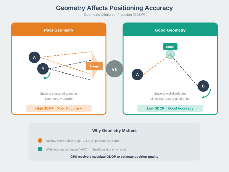
Use GDOP as a review signal:

position_uncertainty ~= range_uncertainty * geometry_factor + environment_bias + timing_bias + filter_lag

The geometry factor is not the whole error budget, but it is a useful warning sign. If the geometry factor is high, improving firmware or filter settings may not fix the installation. Move anchors, add viewing angles, or reduce the area claimed by that anchor group.

Use a simple coordinate example. A 30 m x 20 m work area might use anchors at known map coordinates and a tag mounted on a cart. If the cart is near the middle, several anchors may see it from different angles and a 0.20 m range error may stay near that scale in the final position. If the same cart moves outside the anchor hull or all useful anchors are on one side, geometry can amplify that same range error. With a geometry factor of 3, the review should expect about 0.20 m x 3 = 0.60 m of position uncertainty before adding environment bias, clock error, or filter lag. GDOP does not predict every error; it warns when the installation makes small timing errors expensive.

Good anchor layouts usually follow these principles:

• Surround the area instead of placing every anchor on one side.
• Keep enough independent anchor visibility at the edges and corners, not only in the center.
• Place anchors high enough to reduce obstruction, but not so high that horizontal geometry becomes weak.
• Use height diversity for 3D estimates and for tall workspaces.
• Recompute geometry when walls, racks, machines, or anchor locations change.

34.9 Measurement Quality Pipeline

UWB systems produce timed observations first. A positioning engine turns those observations into an estimate only after filtering poor measurements, solving the geometry, and assigning quality.

UWB positioning measurement pipeline from raw time observations through quality checks, anchor selection, solver, residual review, confidence class, and application policy.

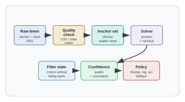
Review each stage:

• Raw observation: Capture timestamp, anchor ID, channel/profile, received signal indicators, sequence number, and clock status where available.
• Quality check: Mark likely NLOS, stale, inconsistent, or missing observations before solving position.
• Anchor selection: Prefer diverse anchors with compatible timing and line-of-sight evidence.
• Solver: Estimate position and calculate residuals or consistency checks.
• Filter: Smooth motion without hiding jumps, blocked anchors, or stale data.
• Confidence class: Publish a confidence label and uncertainty estimate with the position.
• Application policy: Decide whether the estimate is good enough for display, logging, automation, or safety-related action.

This pipeline prevents a common failure: a location server publishes a coordinate even when the underlying evidence is weak, and the application treats the coordinate as certain.

Publish coordinates with confidence, update age, anchors used, and residual evidence. A coordinate without quality fields is not enough for automation or safety decisions.

34.10 Architecture Choices

Choose the architecture from the workflow, scale, update behavior, wiring constraints, and evidence needs. Avoid selecting a mode only because a demonstration kit makes it easy.

UWB positioning architecture choices comparing TWR, TDoA, and angle-assisted approaches by tag behavior, anchor needs, synchronization, solver evidence, and likely fit.

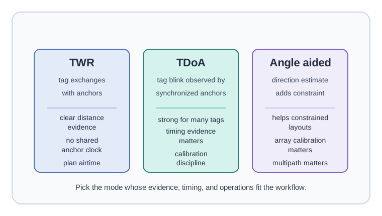
TWR positioning uses message exchanges between a tag and anchors. It is straightforward to reason about because each distance estimate comes from an exchange with a known anchor. It can be a good fit for smaller systems, commissioning, peer distance checks, or systems where synchronized anchor timing is not available. The trade-off is that tags and anchors spend airtime on each exchange, so update rate and tag count must be planned.

TDoA positioning lets a tag transmit a short blink observed by synchronized anchors. It can scale better when many tags report periodically because the tag does not have to range with each anchor. The trade-off is that anchor timing, cabling or timing distribution, calibration, and timestamp quality become part of the position evidence.

Angle-assisted positioning adds direction estimates from antenna arrays or phase information. It can help in constrained layouts, but it introduces its own calibration and multipath sensitivity. Treat angle evidence as another measurement with quality, not as a replacement for line-of-sight review.

34.11 Try Angle of Arrival in the Workbench

34.12 Capacity Often Picks the Positioning Method

The reason large deployments often favor TDoA over TWR is channel airtime. In TWR, every position needs a back-and-forth exchange between the tag and each anchor, so airtime scales with tags x anchors x update rate. In TDoA, a tag transmits one blink and synchronized anchors listen, so one short transmission can support the fix. That is why asset-tracking systems with many tags often lean TDoA, while a smaller set of high-accuracy robots or tools may afford TWR.

Capacity belongs in the same evidence record as geometry. If 200 tags need a 1 Hz update, the system must budget about 200 tag reports per second before retries, management frames, and rejected observations. If the workflow can accept 0.2 Hz for slow-moving assets, the load drops to 200 x 0.2 = 40 reports per second. That change may decide whether TDoA blinks are sufficient, whether TWR exchanges are practical only for a smaller tool fleet, or whether the project needs smaller zones with different update policies.

Compare two rough budgets. In a TWR design with 80 active tags, 4 anchors per position, and 1 update per second, the system asks for about 80 x 4 x 1 = 320 tag-anchor ranging exchanges per second. If a commissioning mode uses only 10 tools at 2 Hz, the request is 10 x 4 x 2 = 80 exchanges per second, which may be more manageable and gives each tool stronger per-anchor evidence. In a TDoA design, 80 tags at 1 Hz can be closer to 80 tag transmissions per second because synchronized anchors listen to the same blink. The tradeoff is that anchor synchronization, timestamp quality, and calibration become release-critical evidence.

The solver then turns accepted observations into position with an error budget, not a guarantee. A practical record might say: range uncertainty 0.15 m, geometry factor 2.5, expected environment bias 0.20 m, and filter lag allowance 0.10 m. A simple review estimate is 0.15 x 2.5 + 0.20 + 0.10 = 0.675 m. If the application needs only room-level asset awareness, that may be acceptable. If it needs a robot safety boundary at 0.30 m, the same evidence is not good enough.

Architecture review questions:

• How many tags may be active in the same area at peak load?
• What update rate is required, and what happens when updates are delayed?
• Can anchors share a reliable timing reference?
• Does the application need a position, a zone, a direction, or a confidence class?
• What fields will be exposed when the engine rejects an estimate?
• Which physical changes require retesting?

34.13 Site Survey and Deployment Process

A site survey should produce an installable coordinate system and an evidence trail. It is not just a count of anchors.

UWB positioning deployment review flow from requirements through coordinate frame, obstruction survey, anchor plan, calibration, acceptance tests, release evidence, and retest triggers.

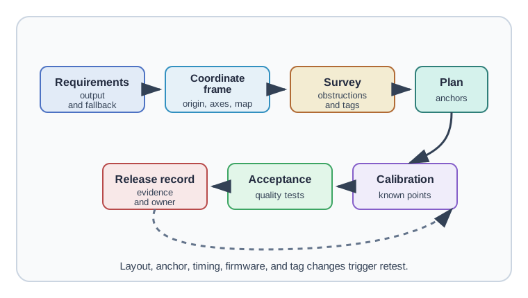
Minimum survey outputs:

• Coordinate frame origin, axes, units, floor level, and map reference.
• Anchor candidate positions with height, mounting surface, orientation, and service access.
• Obstruction notes for metal, water, machinery, people flow, doors, vehicles, and moving fixtures.
• Expected tag mounting positions and body or asset shadowing risks.
• Measurement mode, update policy, timing source, and channel/profile settings.
• Calibration path or reference measurements used to verify the coordinate frame.
• Acceptance zones with expected confidence, residual limits, and update-age limits.
• Retest triggers for anchor movement, new shelving, changed tag mounting, firmware changes, or timing-source changes.

Acceptance testing should include both positive and negative cases:

• Known points near the center, edges, corners, and obstruction boundaries.
• Moving paths at realistic speeds.
• Temporary anchor loss and recovery.
• NLOS conditions that should lower confidence or reject the estimate.
• Neighboring zones where a tag should not be accepted as inside the wrong area.
• Application behavior when the estimate is stale or low confidence.

34.14 Worked Design Review

Consider a warehouse that needs to locate tagged carts on a floor with tall shelving and moving vehicles. A weak review asks, “How many anchors do we need?” A stronger review asks, “Which positions can see enough independent anchors, what evidence proves the estimate quality, and what does the application do when the estimate is weak?”

A practical review sequence:

1. Define the required output as a zone, 2D coordinate, 3D coordinate, or motion track.
2. Choose acceptance metrics such as maximum update age, minimum visible anchors, residual threshold, and confidence class.
3. Draw the coordinate frame and mark shelves, doors, workcells, vehicle paths, and likely tag mounting heights.
4. Place candidate anchors to surround the operating area and to preserve visibility at edges.
5. Simulate or sample geometry quality across the floor.
6. Walk test known points and moving paths, saving raw observations and solved estimates.
7. Tune rejection rules before smoothing rules, so the filter does not hide bad measurements.
8. Document the release record and retest triggers.

The output is not only a map. It is a repeatable evidence package that explains where the system is trustworthy, where it is degraded, and where the application should fall back.

34.15 Knowledge Check

34.16 Capacity Check

34.17 Matching Review

34.18 Deployment Sequence Review

34.19 Common Review Failures

Treating accuracy as a fixed product property: Position quality changes with geometry, line-of-sight, mounting, timing, update rate, and filtering. Publish confidence instead of only a coordinate.

Accepting coordinates without raw evidence: Keep raw measurements, anchors used, residuals, and rejected-anchor reasons so field problems can be reproduced.

Optimizing the center and ignoring edges: Edges, corners, doorways, lifts, racks, and vehicle paths often have weaker geometry than the open middle of a room.

Hiding NLOS with smoothing: Filters can make bad data look stable. Reject weak measurements first, then smooth accepted estimates.

Forgetting the coordinate frame: A precise tag estimate is useless if the anchor map, floor level, axis direction, or application map is misaligned.

34.20 Plain Sources

• IEEE 802.15.4z-2020.
• FiRa Consortium technical materials on UWB ranging and interoperability.
• Indoor Positioning and Indoor Navigation survey literature.
• UWB RTLS deployment and calibration guides from equipment manufacturers.

34.21 Summary

UWB positioning design is an evidence problem. A useful deployment records anchor coordinates, measurement quality, geometry, timing, calibration, confidence, and application behavior. The best systems do not simply claim precision; they explain when estimates are trustworthy, when confidence should fall, and which physical changes require retesting.

Key takeaways:

• Anchor geometry controls how measurement errors are amplified.
• TWR, TDoA, and angle-assisted modes have different evidence and infrastructure needs.
• Line-of-sight, timing quality, and residual checks should be visible to the application.
• Acceptance tests must include weak areas, motion paths, NLOS cases, and stale estimates.
• Retest whenever anchors, tags, maps, timing, firmware, or the physical layout changes.

34.22 What’s Next

• UWB Applications and Security - Apply positioning evidence to practical UWB workflows and risk reviews.
• UWB Ranging Techniques - Review the measurement methods used by positioning engines.
• UWB Fundamentals - Revisit the radio behavior behind UWB measurement quality.
• NFC Fundamentals - Compare deliberate tap workflows with continuous location evidence.
• RFID Design and Deployment - Compare RFID deployment evidence with UWB positioning evidence.