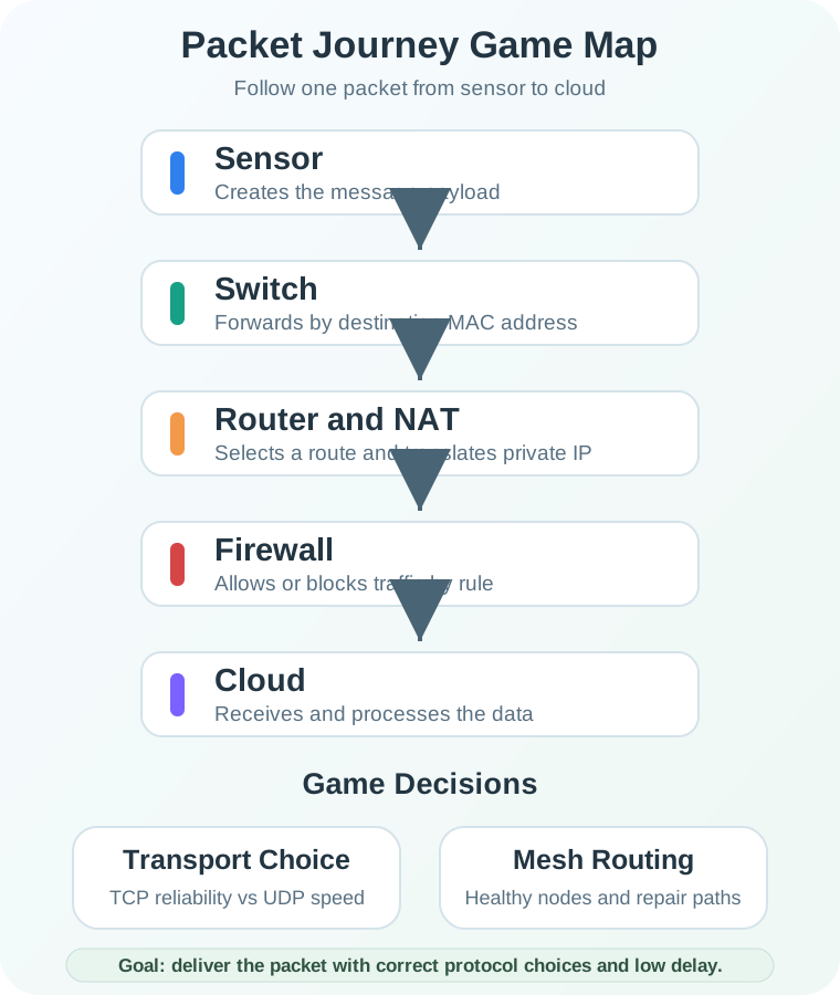
The packet journey game works because it turns hidden forwarding decisions into visible choices. A sensor message has to leave its local link, cross devices that make forwarding decisions, and arrive with enough context for the application to understand it.
Treat each game move as a real deployment question. Which address is used here? Which device decides the next hop? What delay or loss did the packet collect? That habit makes the game a rehearsal for debugging.
Chapter Roadmap
Follow the packet journey from play to proof:
First use the game to separate LAN switching, WAN policy, and IoT mesh choices.
Then read the delay examples as evidence that each hop and retry changes the final mission result.
Next turn the score into a path proof with labels, trace fields, and owner decisions.
Finally connect the same reasoning to troubleshooting, summary review, and the chapters that follow.
Checkpoints recap the route; collapsed sections and the embedded game carry the extra detail.
Key Concepts
Gamification: Applying game design elements (scoring, challenges, feedback) to educational content to increase engagement and retention
Knowledge Check Game: An interactive exercise where correct answers to networking questions unlock subsequent levels or earn points
Immediate Feedback: Providing the correct answer and explanation right after a wrong response, accelerating learning compared to end-of-module feedback
Spaced Repetition: Presenting concepts at increasing intervals to strengthen long-term memory; implemented in some game-based learning tools
Scenario Simulation: A game format that presents a realistic IoT deployment problem and scores the player’s design or troubleshooting decisions
Difficulty Progression: Starting with simple recall questions and advancing to complex scenario analysis as the player demonstrates mastery
Leaderboard: A competitive element showing relative scores among classmates; motivates engagement but should be used carefully to avoid discouraging struggling students
7.2 In 60 Seconds
Guide a data packet from source to destination in this interactive game, making routing decisions across three network environments. Apply OSI layer knowledge, select correct protocols, and overcome real-world challenges like congestion, node failures, and firewalls while learning packet encapsulation and forwarding mechanics.
Phoebe’s Field Notes: Why the “Shorter” Mesh Hop Can Be the Worse Hop
Phoebe’s Why
Level 3’s RPL challenge picks the higher-battery node over the shorter path, and the game is right for a second, physical reason it doesn’t state: distance alone does not set how much signal a mesh hop loses. An isotropic radio’s power spreads over an ever-growing sphere, so even in free space, loss climbs with distance squared. Real indoor hops – past furniture, soil, damp walls, a sensor mounted near the ground – lose faster than that, because scattering and absorption add their own toll. The log-distance model captures this with one number, the path-loss exponent \(n\): a clear hop might sit near \(n=2\), a cluttered one well above it, so two hops of the same length can differ by many decibels. That is the physical face of “low RSSI problem” in this chapter’s troubleshooting list, and it is why RPL’s local repair sometimes has to accept a route with a worse latency number, like the 50 ms alternate path, rather than keep a link whose margin has collapsed.
The Derivation
Inverse-square spreading of transmit power \(P_t\) over a sphere of radius \(d\):
\[S = \frac{P_t}{4\pi d^2}\]
Free-space path loss, adding an isotropic receive aperture \(\lambda^2/4\pi\):
Link margin above receiver sensitivity \(S_{rx}\), the number RPL’s routing metric is really reading:
\[M = P_t - \mathrm{PL}(d) - S_{rx}\]
Worked Numbers: Two Hops, Same Distance
The game names no radio or RF distance, so the worked numbers use catalog-typical 2.4 GHz mesh figures (\(f=2.45\) GHz, \(\lambda=0.122\) m, \(+8\) dBm output, \(-97\) dBm sensitivity) at the same 20 m hop length, comparing only the environment:
\(\mathrm{FSPL}(d_0{=}1\text{ m}) = 20\log_{10}(4\pi/0.122) = 40.2\) dB
Open indoor hop (\(n=2.2\), catalog-typical lightly obstructed): \(\mathrm{PL} = 40.2 + 10(2.2)\log_{10}(20) = 68.8\) dB, margin \(= 8-68.8-(-97) = 36.2\) dB
Cluttered near-ground hop (\(n=3.6\), catalog-typical for furniture, soil, and damp walls at sensor height): \(\mathrm{PL} = 40.2 + 10(3.6)\log_{10}(20) = 87.1\) dB, margin \(= 8-87.1-(-97) = 17.9\) dB
Same 20 m, different environment:\(87.1-68.8 = 18.2\) dB lost to clutter alone – nearly half the clean hop’s margin, from an exponent difference the “hop count” in the game board never shows
A radio’s RSSI reading is itself an integer-dBm, quantized measurement (catalog-typical 1 dB steps from the receiver’s logarithmic detector), so an 18 dB gap like this one is unmistakable to RPL’s link metric, while a 1 dB difference between two struggling links can sit inside the measurement’s own quantization step – one more reason a routing decision needs a fade-margin number, not just a hop count.
Quick Check: Packet Forwarding Choice
7.3 Learning Objectives
By the end of this chapter, you will be able to:
Apply networking concepts in an interactive game environment by guiding a packet through LAN, WAN, and IoT mesh levels
Analyze packet routing decisions across different network types including switched LANs, routed WANs, and 6LoWPAN mesh networks
Select correct protocols at each OSI layer based on reliability, latency, and energy constraints in real-time scenarios
Differentiate between Layer 2 and Layer 3 forwarding by explaining when switches use MAC addresses versus when routers use IP addresses
Evaluate the impact of protocol choices on end-to-end latency by calculating delay budgets across multi-hop paths
Construct an understanding of packet encapsulation by tracing how headers are added, compressed, and removed at each network boundary
For Beginners: The Packet Journey Game
This interactive game lets you experience networking by playing the role of a data packet traveling through a network. You will make decisions about routing, deal with congestion, and learn how real networks work—all through a fun, game-based experience that requires no prior technical knowledge.
Sensor Squad: Become a Packet!
“This is so cool—you get to BE a data packet!” exclaimed Sammy the Sensor. “You travel through the network, hopping from router to router, making decisions at every stop!”
“At each hop, you have to choose the right path,” explained Max the Microcontroller. “Take the wrong route and you might hit congestion, a firewall, or a failed node. It is like a maze where you need to apply everything you know about network layers and routing.”
Lila the LED was already playing. “I just learned that picking UDP instead of TCP at the transport layer makes my packet faster but riskier—no retransmission if I get lost! And at each router, I need to check the routing table to find the best next hop.”
“The game has three levels that get harder,” said Bella the Battery. “Level 1 is a simple home network, Level 2 is a campus with multiple subnets, and Level 3 is a full internet journey with firewalls and NAT. See how many packets you can deliver without losing any lives!”
The setup has named the player and the three levels. The next question is what the game asks the packet to prove at each boundary.
7.4 Packet Journey Adventure
Time: ~20 min | Difficulty: Intermediate | Unit: P07.C15.U10
Learn Networking by Adventure
Guide a data packet from source to destination across three increasingly complex network environments. Make correct routing decisions, apply the right protocols at each layer, and overcome network challenges like congestion, failures, and firewalls.
Putting Numbers to It
Every routing choice in the game changes end-to-end delay.
Question: In Level 1 of the Packet Journey game, a switch must forward a frame to a device on the same LAN. Which address does the switch use?
Answer: The switch uses the destination MAC address, because switches forward at OSI Layer 2. IP addresses are used by routers at Layer 3, and port numbers belong to Layer 4.
Packet Journey Adventure
Guide one sensor packet through LAN, WAN, and IoT mesh decisions.
LevelReady
Score0
Latency0 ms
Retries3
Checkpoint: Three-Level Route
You now know:
Level 1 asks whether local forwarding uses MAC addresses, routes, and NAT correctly.
Level 2 adds transport choice, QoS priority, and firewall order.
Level 3 adds 6LoWPAN compression, RPL energy choice, repair, and border-router decompression.
The game has made the route visible. The next question is whether the route still meets a time budget when hops, queues, and retries are counted.
Learning Objectives Covered in This Game
The Packet Journey game reinforces these key networking concepts:
Level 1 - LAN Routing:
MAC vs IP Addressing: Switches use MAC addresses (Layer 2), routers use IP addresses (Layer 3)
NAT Traversal: How private IPs are translated to public IPs for internet communication
Routing Tables: How routers determine next hop based on destination IP
Level 2 - WAN Routing:
TCP vs UDP: When to use reliable (TCP) vs low-latency (UDP) transport
QoS Prioritization: How critical traffic gets priority during congestion
Firewall Rules: How stateful firewalls inspect and filter packets
Level 3 - IoT Mesh Routing:
6LoWPAN: Header compression for constrained IPv6 networks
RPL Routing: Energy-aware routing protocol for IoT mesh networks
Failure Recovery: How mesh networks reroute around failed nodes
Header Encapsulation/Decapsulation: Protocol processing at border routers
Quick Check: Leaving a 6LoWPAN Mesh
Question: When a packet leaves a 6LoWPAN mesh through a border router, compressed headers are restored to full IPv6 format. What is this process called?
Answer: This is header decompression. 6LoWPAN compresses IPv6 headers inside the constrained mesh, and the border router expands them back to standard IPv6 format for external networks.
Packet Delay Budget Analysis
Scenario: You’re designing a smart traffic light system. When a pedestrian presses the crosswalk button, the traffic controller must receive the signal within 500 ms to meet safety standards.
Network Path (similar to Game Level 2):
Step
Network point
Role in the journey
1
Sensor button
Creates the safety message.
2
Edge router
Forwards the packet out of the local network.
3
ISP core
Carries the packet across the provider network.
4
Peering point
Hands traffic between networks; congestion often appears here.
5
Cloud firewall
Checks whether the packet is allowed.
6
Traffic controller
Receives the message and changes the crossing state.
Delay Components from Packet Journey Game:
Hop 1: Sensor to Edge Router (LAN)
Physical propagation: ~0 ms (100 m at ~2×10^8 m/s in copper ≈ 0.0005 ms, negligible)
MAC layer (CSMA/CA): 5 ms average (Wi-Fi contention + backoff)
Processing delay: 2 ms (edge router forwarding + queuing)
Hop 1 Total: 7 ms
Hop 2: Edge Router to ISP Core
Propagation: 10 ms (fiber link to ISP, 2,000 km at 2×10^8 m/s)
Transmission delay: 0.12 ms (1,500 byte packet at 100 Mbps = 12,000 bits ÷ 10^8 bps)
Queueing delay: 14.88 ms (router processing typical load)
Hop 2 Total: 25 ms
Hop 3: ISP Core to Peering Point
Propagation: 20 ms (cross-country fiber)
QoS decision: 5 ms (Level 2 challenge - classify as “critical alarm”)
Queueing: 30 ms (congested peering point during evening peak)
Hop 3 Total: 55 ms
Hop 4: Peering Point to Cloud Firewall
Propagation: 15 ms
Firewall inspection: 2 ms (Level 2 challenge - rule matching)
Hop 4 Total: 17 ms
Hop 5: Cloud Firewall to Traffic Controller
Propagation: 5 ms (local data center)
Application processing: 10 ms (TLS decryption + application logic)
Hop 5 Total: 15 ms
Total End-to-End Delay and Safety Margin:
Check
Calculation
Result
Total path delay
7 + 25 + 55 + 17 + 15
119 ms
Safety budget
System requirement
500 ms
Remaining margin
500 - 119
381 ms of headroom
Design status
119 ms < 500 ms
Within the safety budget
What If We Made Wrong Protocol Choices?
Bad Decision 1: Skip QoS (treat as best-effort traffic) - Peering point queueing increases from 30 ms to 200 ms during congestion - New total: 119 - 30 + 200 = 289 ms (still OK, but margin reduced to 42%)
Bad Decision 2: Use UDP instead of TCP (Game Level 2 choice) - 5% packet loss requires retransmission - Retransmit timeout: 200 ms (RTT × 2) - Expected delay: 119 ms × 0.95 + (119 + 200) × 0.05 = 129 ms average - But worst-case (packet lost): 319 ms (still within 500 ms)
Bad Decision 3: Firewall rule misconfiguration (Game Level 2) - Packet blocked by default deny rule - Sensor timeout + retransmit: 1,000 ms (exceeds safety budget) - System failure: Pedestrian button press not detected
Real-World Lesson from Game Mechanics:
The Packet Journey Game teaches that delay is cumulative and unpredictable: - Each hop adds latency (sum of all hops) - Wrong protocol choices (UDP without retries, best-effort QoS) add risk - Firewall errors cause complete failure, not just delay
Design Rule: Budget for worst-case, not average: - Average path: 119 ms - Worst-case (congestion + 1 retransmit): ~500 ms - Design with 2x safety margin: 500 ms requirement means a 250 ms target latency
If using wireless sensors, avoid multi-hop mesh (each hop adds 10-50 ms)
Game shows RPL mesh with 4 hops = 50+ ms total just for mesh routing
Better: Direct Wi-Fi to edge router (single hop = 7 ms)
Final System Design:
Segment
Design choice
Typical delay
Sensor to edge router
Direct Wi-Fi, single hop
7 ms
Edge router to ISP core
QoS enabled
25 ms
ISP core to cloud
Expedited Forwarding
35 ms
Cloud to controller
Firewall pre-configured
32 ms
Total
Typical path
About 99 ms
Safety requirement
Worst-case design target
About 350 ms worst-case, still below 500 ms
Key Insight from Game: Protocol decisions at each layer (MAC, transport, network, application) compound across the entire path. The game’s level structure mirrors real network hops, teaching that every decision matters for end-to-end latency.
Checkpoint: Delay Budget
You now know:
The worked path totals 119 ms, leaving 381 ms inside a 500 ms safety budget.
Skipping QoS, losing a packet, or blocking at the firewall changes the mission differently.
A direct Wi-Fi hop can keep the sensor-to-edge segment near 7 ms.
The timing story is now concrete. The next task is to label the packet journey so each decision has a visible place in the trace.
Match: Game Concept to OSI Layer
Order Sensor-to-Cloud Packets
Common Pitfalls
Review Wrong Game Answers
Replaying a game to improve the score without reading the explanations for wrong answers reinforces incorrect mental models. Fix: read every explanation carefully before attempting the next question, even when the answer was correct.
2. Treating a High Game Score as Mastery
Game scores measure performance on a specific question set, not broad mastery. Fix: supplement game exercises with worked examples, labs, and scenario problems to confirm genuine understanding.
Treat the Game as Required
Interactive games in this module are designed to reveal common misconceptions that text alone may not expose. Fix: attempt every game exercise and use wrong answers as diagnostic information about which concepts need more study.
Label the Diagram
Code Challenge
7.5 Knowledge Check
7.6 Packet Journey Path Proof
The packet journey game is more than a score. Each choice asks the learner to prove that a packet can move through one boundary without losing the meaning of the previous boundary. A switch proves local delivery with MAC forwarding, a router proves network delivery with IP next-hop choice, and the end system proves that the application result still arrived.
Figure 7.1: Packet journey game map from sensor message through switch, router and NAT, firewall, cloud, transport choice, and mesh routing decisions.
The useful score is not just delivery. It is the evidence trail from payload creation through forwarding, policy, transport choice, and final receiver behavior.
That is the same habit used in real IoT troubleshooting: trace the packet from source intent to link behavior, network route, transport trade-off, security check, and receiver outcome. The game makes the boundary visible because every level asks a different kind of question. A local LAN question asks whether a frame reached the right neighbor. A WAN question asks whether a route, NAT mapping, or firewall rule allowed the flow. A mesh question asks whether the path still works when a low-power node changes parent or needs a repair path.
The important review move is to separate arrival from proof. A packet that eventually reaches the cloud may still be a bad design if it spent too much time in link retries, crossed a fragile NAT state, relied on a firewall exception that is not documented, or consumed a battery-heavy mesh repair. The path proof says what each layer contributed and where the next real test belongs.
When a learner can explain the game route this way, the lesson transfers to commissioning work. The operator does not say only “the packet failed.” The operator asks which boundary was last proven: payload creation, neighbor delivery, routed next hop, transport recovery, security policy, or application processing.
That boundary question keeps the game from becoming memorization; every successful move must leave a clue that would still help during a field failure.
Checkpoint: Path Proof
You now know:
Arrival is not enough; each boundary needs evidence.
LAN, WAN, and mesh questions prove different parts of the packet journey.
A useful score leaves clues about retries, NAT state, firewall policy, and receiver behavior.
The proof explains what happened. The trace record turns that explanation into a short artifact another operator can replay.
7.7 Packet Trace Record
After playing a level, turn the route into a small trace record. The record explains why a path was chosen, where delay or loss entered, and which layer owns the next fix. Use the same structure in a real lab with a sensor log, a gateway packet capture, router or firewall counters, and the application or broker log. The goal is not a large report; the goal is a short evidence chain that someone else could replay.
Start with a stable packet identity. In a classroom game that may be the level name and decision sequence. In a deployment it may be a payload sequence number, MQTT message identifier, CoAP token, TCP stream, UDP five-tuple, or timestamped sensor sample. Then record each boundary in order. If two clocks disagree, keep both timestamps and note the clock source rather than forcing a false precision.
Trace Field
What To Record
Layer Boundary
Local link
Source interface, destination MAC or neighbor, link errors, and retry signs.
Layer 2 proves the next local hop, not the full route.
Network route
Destination IP, selected next hop, TTL or hop limit, congestion, and alternate path.
Layer 3 proves reachability between networks and loop control.
Transport choice
Reliability need, retry budget, latency target, and loss tolerance.
Transport behavior decides whether speed or recovery matters more.
Receiver result
Delivery time, dropped packet reason, firewall or NAT decision, and final application result.
The end result proves whether the earlier path decisions were acceptable.
A practical trace also names the owner of the next action. A link retry or low RSSI problem belongs with radio placement, antenna orientation, cabling, or local medium access. A wrong next hop, missing route, expired ARP entry, or bad IPv6 neighbor entry belongs with addressing and routing. A timeout after a lossy hop may belong with transport tuning. A denied flow belongs with firewall policy, NAT state, or broker authorization. The game is useful because it trains that ownership split before a live incident.
For IoT systems, add two fields that ordinary web traces often skip: energy effect and freshness effect. A packet can arrive after a mesh repair but drain a sleeping node with extra retransmissions. A dashboard can show the last successful value while the newest sample is delayed or dropped. Recording retry count, hop count, queue delay, and receiver timestamp prevents a false pass when the mission depends on current data.
Checkpoint: Trace Ownership
You now know:
A trace record starts with a stable packet identity and then records each boundary in order.
Link, route, transport, policy, and receiver failures have different owners.
IoT traces should include energy effect and freshness effect, not only final arrival.
With ownership separated, the final under-the-hood view asks why small hop choices can combine into a large delay or failure.
7.8 Small Hop Choices Compound
Each hop can look harmless in isolation. One extra retry, one congested next hop, one firewall detour, or one mesh repair can be acceptable by itself. Across a packet journey, those choices add delay, raise loss probability, and change whether the application result still meets its deadline.
The important under-the-hood idea is that layer decisions compound. A Layer 2 retry consumes time before Layer 3 even chooses the next hop. A transport retry can hide a link problem but increase latency. A firewall or NAT decision can be correct for policy and still break a stateful return path if the session record is missing.
Several hidden tables make the game realistic. A switch uses its MAC address table to select a port. A router uses a forwarding table and decrements IPv4 TTL or IPv6 hop limit. Neighbor discovery or ARP proves the local next-hop address before the frame can leave. NAT and stateful firewalls keep flow state so the return traffic matches an allowed session. In a low-power mesh, RPL parent choice and repair behavior can change the route without the application knowing why.
Those tables age at different speeds. A neighbor cache can expire, a NAT mapping can time out, a firewall state entry can disappear, and a routing protocol can converge after a topology change. The packet journey score hides that timing unless the trace record names which state was fresh at the moment of forwarding. This is why a path can pass once and fail later under sleep cycles, bursts, or gateway outages.
Use the game result as a diagnostic: do not ask only whether the packet arrived; ask which layer made the risky decision, whether the decision was necessary, and what proof would let an operator fix it. A good under-the-hood answer separates propagation delay, serialization delay, queueing, link retransmission, transport recovery, policy inspection, and receiver processing. That separation turns “slow network” into a testable hypothesis about a specific layer boundary.
7.9 Summary
The Packet Journey game demonstrates how every protocol decision compounds across network hops. A wrong transport-layer choice (UDP instead of TCP for critical data), a missing QoS marking, or a misconfigured firewall rule each affects end-to-end latency or causes outright delivery failure. The three-level structure—LAN, WAN, and IoT mesh—shows that the same core principles (addressing, forwarding, encapsulation) apply from a home switch all the way to a battery-constrained 6LoWPAN sensor node.
7.10 What’s Next
You have completed the Networking Fundamentals series. The table below shows where to go next based on the concepts introduced in this game.
Extend the firewall rule challenge from Level 2 into a full study of IoT threat models, packet filtering, and intrusion detection
7.11 Key Takeaway
The packet journey game shows that routing, switching, transport choice, firewall rules, and mesh behavior combine into one end-to-end outcome. A wrong choice at one hop can break the mission.

 Checkpoint: Three-Level Route