flowchart LR
  L[Link evidence<br/>RSSI, cable, association] --> A[Address evidence<br/>IP, mask, lease, gateway]
  A --> G[Gateway evidence<br/>ARP or ND plus ping]
  G --> N[Naming evidence<br/>DNS query and answer]
  N --> T[Transport evidence<br/>port, timeout, TLS]
  T --> S[Service evidence<br/>topic, route, response]
3 Lab: Network Diagnostics
networking-core
3.1 Start With the First Broken Boundary
A networking lab is not a hunt for random commands. It is a way to find the first boundary where a device stops meeting its promise: link joined, address assigned, gateway reachable, name resolved, port open, service responding.
Read the lab outputs like a short investigation. Each measurement should let someone else see why you moved up the stack, stopped at a fault, or ruled out a tempting but wrong explanation.
3.3 Learning Objectives
By the end of this chapter, you will be able to:
- Build Network Diagnostics Tools: Construct ESP32 and Python network analysis tools that report IP, RSSI, subnet, and gateway information
- Analyze Network Configurations: Apply Python to calculate subnets, interpret IP address components, and evaluate network boundaries using bitwise operations
- Troubleshoot Connectivity Problems: Diagnose network failures by applying a systematic 5-step diagnostic flow across OSI layers
- Evaluate Protocol Security: Differentiate between secure and insecure IoT ports and select appropriate encrypted alternatives for production deployments
- Summarize Core Networking Terms: Explain key networking concepts including IP addressing, MAC addresses, DNS, DHCP, and NAT using the provided glossary
For Beginners: Networking Labs
Labs are where you learn by doing. In these exercises, you will build small networks, test connections between devices, and troubleshoot problems – much like a mechanic learns by working on actual engines. No prior networking experience is needed; each lab walks you through step by step.
Chapter Roadmap
This lab chapter is long, so use it as a guided investigation:
- First learn the evidence ladder: signal, address, gateway, DNS, transport, then service.
- Then practice the 5-step diagnostic flow with browser dashboards before touching hardware.
- Next build evidence packets for ESP32, subnet, ARP or neighbor discovery, and scanner labs.
- After that review the networking fundamentals that make the lab results meaningful: IPv6, UDP vs TCP, ports, NAT, topology, and RSSI.
- Finally use the quizzes, pitfalls, and code challenge to prove you can explain the first failed boundary.
Checkpoints recap what you have already proven. Collapsed callouts and galleries are useful deepening material, but the main path is the evidence chain.
3.4 Overview: Diagnostics Follow Evidence
The first question is not “which command should I run?” It is “which boundary am I trying to prove?” Start by separating radio, addressing, routing, naming, transport, and service evidence.
A networking lab is useful only when each observation narrows the fault. Start with local physical or radio evidence, then IP configuration, then local gateway reachability, then naming, then transport reachability, then the application service. The goal is not to collect every possible metric; it is to build a chain of proof that shows where the path first stops behaving as expected.
That order prevents a common mistake: blaming the cloud, MQTT broker, or device firmware before proving the device has a stable signal, valid address, reachable gateway, and working resolver. If the device has poor RSSI or a flapping Ethernet link, a DNS error is only a later symptom. If DHCP failed, testing an MQTT topic wastes time because the device does not yet have a usable network identity. If the gateway is reachable but DNS fails, the service owner is not the first responder. The lab should teach students to say, “this layer is proven enough to move up” or “this layer is the first failed boundary.”
For example, an ESP32 that says “cloud unavailable” may actually have four different root causes. It may be associated with Wi-Fi but sitting at -82 dBm, causing retries and timeouts. It may have a self-assigned address because the DHCP exchange failed. It may have a valid address but no route outside the subnet. It may reach the gateway but fail DNS because the resolver address is wrong. Only after those checks pass does an MQTT broker, REST endpoint, TLS certificate, or application credential become the likely cause. The overview lesson is that each lab output is evidence for a boundary, not a generic success or failure light.
3.5 Diagnostic Packet
For each lab run, record the timestamp, device identity, firmware or script version, SSID or lab network, RSSI or link state, local IP, subnet mask, gateway, DNS server, first gateway test, first name-resolution test, first transport test, and first service test. That packet lets another person replay the diagnosis without guessing what was observed. It also prevents students from editing three variables at once and then claiming a fix without knowing which variable mattered.
A practical record should include both the command and the result. “Ping gateway failed” is better than “network broken”; “DNS query for broker.example.test timed out while ping to 192.168.1.1 succeeded” is better still. When using ESP32 code, print the Wi-Fi status, RSSI, local IP, gateway, DNS server, and elapsed time for each test. When using a laptop or VM, pair ip addr, ip route, arp -a or ip neigh, dig, nc or curl, and a packet capture. The tool names may change by platform, but the evidence categories stay stable.
When a step fails, stop and explain the boundary. Weak RSSI points at placement, antenna orientation, channel congestion, or enclosure effects. A 169.254.x.x address on many systems points at address self-assignment after DHCP did not complete. A reachable gateway with failed DNS points at resolver configuration, firewall policy, or upstream name service. A successful TCP connection with an HTTP 401 response is no longer a network reachability failure; it is an authentication or application-policy result. A refused TCP port can mean the host is reachable but no service is listening on that port, which is very different from a route failure.
The most useful lab habit is to preserve the first failure, not only the final fix. If a student changes the SSID password, moves the antenna, restarts the router, and edits DNS in one pass, the lab teaches superstition. If the record shows “DHCP request sent, no offer observed; after gateway DHCP service restart, lease received with mask and DNS,” the class learns an actual diagnostic pattern. That is why the diagnostic packet should be small, timestamped, and repeatable.
3.6 One Symptom, Several Layers
“Cannot reach the server” can mean radio loss, missing DHCP lease, wrong subnet mask, stale ARP or neighbor state, blocked DNS, closed TCP port, failed TLS, rejected credentials, or an application outage. The packet trace is different in each case. A Wi-Fi association failure may show no IP traffic at all. A DHCP failure shows discovery or request messages without a useful lease. A wrong subnet mask can make the device ARP for a remote host as if it were local, or send traffic to the wrong gateway. A stale neighbor entry can produce local delivery attempts that never reach the router. A DNS failure may show UDP or TCP queries but no valid answer. A closed port gives a different signal from a filtered port, and both differ from a TLS alert or HTTP error.
The lab sequence works because lower-layer state gates higher-layer meaning. A port scan result is not actionable until local addressing and routing are known; a DNS failure is not actionable until gateway reachability is proven; a cloud API error is not actionable until transport connection evidence is visible. This does not mean every incident must be debugged slowly from layer 1 every time. It means that the record must show which lower assumptions are already proven, especially when the failure crosses team boundaries between firmware, network operations, cloud service, and application owners.
Under the hood, each boundary has a different state machine. Wi-Fi association proves the station and access point agreed to link-layer participation, but it does not prove DHCP. DHCP proves the device received an address lease and options, but it does not prove the address is useful for the intended route. ARP or IPv6 Neighbor Discovery proves a next-hop link-layer mapping, but it does not prove the next hop forwards traffic. DNS proves a name can resolve to an address, but it does not prove the address accepts the expected transport session. TCP or UDP behavior proves some path and policy properties, but it does not prove the payload is semantically valid for the service.
That separation is why a good lab asks students to annotate the packet trace rather than just run commands. A single failed dashboard tile should be decomposed into evidence: link joined, lease received, gateway resolved, gateway reached, name resolved, port reached, TLS accepted, request authorized, response parsed. Once those checkpoints are visible, troubleshooting becomes a search for the first broken contract instead of a list of guesses.
 Checkpoint: Evidence Order
You now know:
- The lab climbs from link evidence to address, gateway, naming, transport, and service evidence.
- A 169.254.x.x address points at address self-assignment after DHCP did not complete.
- A TCP refusal, TLS alert, HTTP 401, and DNS timeout are different first-failed boundaries, not the same “network down” result.
3.7 Prerequisites
Before diving into this chapter, you should be familiar with:
- Networking Basics: Introduction: Core networking concepts
- Networking Basics: Protocols and MAC: Protocol layers and MAC classification
- Networking Basics: Hands-On Configuration: Configuration, troubleshooting, and security basics
Network Diagnostics Dashboard
The ESP32 network diagnostics tool provides real-time visibility into your IoT device’s network health:
Step 1: Wi-Fi Connection
- Device scans for available networks using
WiFi.scanNetworks() - Authenticates using WPA2 credentials
- DHCP client requests IP address from router
Step 2: Network Information Gathering
WiFi.localIP()queries DHCP-assigned addressWiFi.subnetMask()determines network rangeWiFi.gatewayIP()identifies default routerWiFi.dnsIP()locates DNS resolver
Step 3: Signal Quality Assessment
- RSSI (Received Signal Strength Indicator) measured in dBm
- Values closer to 0 indicate stronger signal
- Categorized: Excellent (>-50), Good (-50 to -60), Fair (-60 to -70), Poor (<-70)
Step 4: Network Calculations
- Network address: IP AND subnet mask (bitwise)
- Broadcast address: IP OR (NOT subnet mask)
- These identify network boundaries and broadcast domain
Run it: Step 4 turns an address and mask into a network and broadcast with bitwise math – do it live in the subnet calculator below. Load a preset such as Sensor VLAN /26 or Factory LAN /24, then step through Network AND and Broadcast to watch the Dotted decimal and CIDR mask resolve into a Usable range and Route decision. Change the prefix and see how the boundary the dashboard reports moves, so a wrong mask like the /30 case elsewhere in this lab becomes obvious before it breaks routing.
Step 5: Connectivity Verification
- DNS test resolves google.com to verify internet access
- Successful resolution confirms gateway routing and DNS functionality
Phoebe’s Field Notes: Why dB Link Margins Add

3.7.1 Phoebe’s Why
The dashboard uses negative RSSI numbers because radio receivers are comparing tiny powers against a fixed one-milliwatt reference. A dB value is not another linear unit; it is a logarithm. That is why link budgets add transmitter power, antenna gain, path loss, obstruction loss, receiver sensitivity, and margin in dB even though the underlying powers multiply and divide. The useful habit is to keep two questions separate: how many dB above sensitivity is the receiver, and what power ratio does that dB gap really mean?
3.7.2 The Derivation
Start with the absolute dBm reference:
\[P_{\mathrm{dBm}} = 10\log_{10}\left(\frac{P_{\mathrm{mW}}}{1\ \mathrm{mW}}\right)\]
Invert it to recover power:
\[P_{\mathrm{mW}} = 10^{P_{\mathrm{dBm}}/10}\]
A dB change is a power ratio:
\[\Delta_{\mathrm{dB}} = 10\log_{10}\left(\frac{P_2}{P_1}\right)\]
\[\frac{P_2}{P_1} = 10^{\Delta_{\mathrm{dB}}/10}\]
Free-space loss comes from spherical spreading plus antenna aperture:
\[P_r = P_tG_tG_r\left(\frac{\lambda}{4\pi d}\right)^2\]
With \(\lambda=c/f\), the path-loss term is
\[L_{\mathrm{FS,dB}} = 20\log_{10}\left(\frac{4\pi df}{c}\right)\]
The link budget is then an addition ledger:
\[P_{r,\mathrm{dBm}} = P_{t,\mathrm{dBm}} + G_{t,\mathrm{dBi}} + G_{r,\mathrm{dBi}} - L_{\mathrm{path,dB}} - L_{\mathrm{extra,dB}}\]
and the usable reserve is
\[M_{\mathrm{dB}} = P_{r,\mathrm{dBm}} - S_{\mathrm{rx,dBm}}\]
3.7.3 Worked Numbers: This Chapter’s RSSI Checks
- Dashboard power at -68 dBm: \(P = 10^{-68/10}\) mW \(= 1.58\times10^{-7}\) mW. The chapter’s excellent reference \(-30\) dBm is \(10^{-30/10}\) mW \(= 1.00\times10^{-3}\) mW.
- The 38 dB gap: \(-30 - (-68) = 38\) dB, so the excellent signal is \(10^{38/10} = 10^{3.8} = 6310\) times the received power. The chapter’s \(41.5\%\) quality value is a dashboard interpolation between \(-95\) and \(-30\) dBm, not a percent of radio power.
- Margin at -68 dBm: with receiver sensitivity \(S_{\mathrm{rx}}=-95\) dBm, \(M=-68-(-95)=27.0\) dB. That is above the chapter’s 15 dB stability target.
- Worst affected sensor: \(M=-85-(-95)=10.0\) dB, so it is \(5.00\) dB short of the 15 dB minimum. Moving from \(-85\) dBm to the chapter’s \(-70\) dBm target is a 15.0 dB improvement and gives \(-70-(-95)=25.0\) dB of margin.
- Power-ratio note: a 10-15 dB RSSI improvement means \(10^{10/10}=10.0\) to \(10^{15/10}=31.6\) times more received power – the chapter’s own “Practical Impact” callout now states this figure directly rather than the earlier \(2.5\)-\(5.6\times\) shorthand, which was not the RSSI power ratio; use the dB formulas above for audit calculations.
Quick-Start Lab Plans: Use these browser-first practice plans before touching hardware code. Each plan tells you what to measure, what result to expect, and what the result means.
Beginner Basic Network Scanner
Objective: Scan your local network and identify active devices.
| Step | What to do | What it teaches |
|---|---|---|
| 1 | Find your device IP address and subnet prefix. | The first three octets often identify a small home or lab network. |
| 2 | Probe a small safe range, such as .1 to .20, not the whole internet. |
Scanning should stay inside networks you own or have permission to test. |
| 3 | Record which addresses respond. | Active hosts usually include the router, your laptop, phones, and IoT boards. |
| 4 | Compare the list after turning one lab device off. | Device discovery is evidence-based: the list should change when the device disappears. |
Expected result: a short device inventory with IP address, likely role, and whether the device is expected in the lab.
Intermediate Service Port Scanner
Objective: Identify which services (HTTP, MQTT, SSH) are running on discovered devices.
| Port | Service | Safe interpretation |
|---|---|---|
| 22 | SSH | Remote administration may be enabled; production devices should use keys and restrict access. |
| 80 | HTTP | A web UI or API may be present; use HTTPS for real deployments. |
| 443 | HTTPS | Encrypted web UI or API. |
| 1883 | MQTT | Plain MQTT broker or client endpoint; acceptable for local testing only. |
| 8883 | MQTTS | MQTT protected by TLS; preferred for production. |
| 5683 | CoAP | Plain CoAP for constrained devices; use DTLS where sensitive data is involved. |
Expected result: a service inventory that connects open ports to likely device functions and security follow-up.
Advanced Network Performance Monitor
Objective: Measure latency, packet loss, and jitter between your device and gateway.
| Metric | Healthy lab target | What to investigate if it fails |
|---|---|---|
| Average latency to gateway | Under 20 ms on local Wi-Fi | Congestion, weak RSSI, overloaded router, or distant access point. |
| Packet loss | 0-1% during a short local test | Radio interference, roaming, or power-saving sleep behavior. |
| Jitter | Small variation between samples | Contention on shared Wi-Fi or unstable mesh path. |
| RSSI | Better than -70 dBm | Distance, antenna placement, metal enclosure, or access-point placement. |
Expected result: a short health report that says whether the issue is radio quality, IP configuration, or application reachability.
3.8 Concept Check: Network Troubleshooting
3.9 Concept Relationships
Understanding how networking concepts interact helps you diagnose issues systematically:
| Concept | Depends On | Affects | Diagnostic Tool |
|---|---|---|---|
| IP Connectivity | Physical link, DHCP | All higher layers | ping gateway |
| DNS Resolution | IP connectivity, DNS server | Application access | nslookup or WiFi.hostByName() |
| RSSI | Distance, obstacles, interference | Packet loss, throughput | WiFi.RSSI() |
| Gateway | Router configuration, routing table | Internet access | traceroute |
| Subnet Mask | Network design | Local vs remote routing | WiFi.subnetMask() |
| NAT | Router configuration | Inbound connections | Port forwarding rules |
Troubleshooting Flow:
- Check physical (RSSI should be > -70 dBm, i.e., Fair or better)
- Verify Layer 2 (MAC address, DHCP)
- Test Layer 3 (ping gateway)
- Check DNS (resolve google.com)
- Test application (HTTP request)
That list is the compact version of the evidence ladder. The simulator below lets you rehearse it under failure conditions before the hands-on labs ask you to collect your own packet.
Checkpoint: Diagnostic Flow
You now know:
- The practical flow has 5 steps: physical, Layer 2, Layer 3, DNS, and application.
- RSSI should be better than -70 dBm, and the chapter’s Wi-Fi examples use a 15 dB link margin as the reliability target.
- If the gateway ping works but DNS fails, the likely failure is resolver configuration or policy rather than Wi-Fi authentication.
3.10 Hands-On Labs
Now turn the diagnostic flow into records. The lab work below is less about writing a long program and more about producing evidence another person can replay.
3.10.1 ESP32 Network Diagnostics Lab
Objective: Create a comprehensive network diagnostics tool on ESP32 that reports all network parameters.
Materials:
- ESP32 development board
- Wi-Fi network
- Serial monitor
Optional ESP32 Diagnostics Build Plan
Use this only after the browser dashboard makes sense. The hardware version should print the same evidence categories, not a long unstructured serial log.
| Build step | ESP32 value to collect | Student check |
|---|---|---|
| Connect to Wi-Fi | Connection status, SSID, channel, RSSI | Did the board associate with the expected 2.4 GHz network? |
| Read IP configuration | Local IP, subnet mask, gateway, DNS | Does the address match the intended lab subnet? |
| Identify hardware | MAC address | Can you match the board to the device inventory? |
| Calculate network boundaries | Network address and broadcast address | Do these match the subnet calculator above? |
| Test reachability | Gateway test and DNS lookup | Is the failure local routing, DNS, or the wider internet? |
Implementation note: if you later write the firmware, keep the output grouped exactly like the table. Students should be able to compare browser simulator results and hardware serial output line by line.
3.11 Consolidated Lab Evidence Packet
Use one evidence packet for the ESP32, addressing, ARP, subnet, and scanner labs:
| Lab thread | Evidence to record | Failure it helps isolate |
|---|---|---|
| ESP32 boot-to-network trace | Association status, DHCP result, IP, subnet, gateway, DNS, MAC, RSSI, and first service attempt | Separates Wi-Fi association from IP configuration and application failures |
| ARP or neighbor discovery | Local IP, MAC address, gateway entry, stale entry age, and refresh result | Shows whether the device can resolve local delivery before blaming the cloud |
| Subnet calculation | IP, mask, network address, broadcast or prefix, usable range, and gateway-in-subnet check | Catches addressing mistakes before port or protocol debugging |
| Port and scanner review | Host, port, protocol, service expectation, refusal or timeout, and firewall note | Distinguishes a closed service from a routing or DNS problem |
Putting Numbers to It
RSSI (Received Signal Strength Indicator) follows a logarithmic scale where every 3 dB change represents a 2× change in power. Calculate signal quality from RSSI measurements.
$ = % $
Worked example: An ESP32 sensor reports RSSI = -68 dBm. The Wi-Fi module’s receiver sensitivity (minimum usable signal) is -95 dBm, and excellent signal is -30 dBm.
Signal Quality = (-68 - (-95)) / (-30 - (-95)) × 100% = (27) / (65) × 100% = 41.5% quality.
Power comparison: -68 dBm = 10^(-68/10) ≈ 0.00000016 mW. Excellent signal at -30 dBm = 10^(-30/10) = 0.001 mW. The excellent signal is 6,310× stronger in absolute power (38 dB difference: 10^(38/10) = 10^3.8 ≈ 6,310).
Practical impact: At -68 dBm, the sensor’s data rate drops to 11 Mbps (from 150 Mbps max) and retransmissions increase by ~15%. Moving 5 meters closer to the access point could improve RSSI by 10-15 dB (10.0-31.6× stronger signal in power, using \(10^{\text{dB}/10}\)), restoring full throughput.
Expected Output Summary:
| Report section | Healthy example | What it proves |
|---|---|---|
| Wi-Fi connection | Connected, RSSI around -45 dBm, channel 6 | Radio link and authentication are working. |
| IP configuration | IP 192.168.1.100, mask 255.255.255.0, gateway 192.168.1.1 | DHCP or static addressing is correct. |
| Hardware identity | MAC address recorded | The physical board can be matched to the inventory. |
| Network information | Network 192.168.1.0, broadcast 192.168.1.255 | Subnet boundaries match the calculator. |
| Connectivity tests | Gateway reachable and DNS resolves a public name | Local routing and DNS are both functioning. |
Learning Outcomes:
- Retrieve all network configuration parameters
- Perform connectivity diagnostics
- Understand Wi-Fi signal strength (RSSI)
- Calculate network and broadcast addresses
- Test DNS resolution
Checkpoint: Evidence Packets
You now know:
- An ESP32 packet should record association status, DHCP result, IP, subnet, gateway, DNS, MAC, RSSI, and first service attempt.
- Subnet checks use the same bitwise operations shown by the calculator: IP AND mask for the network, and IP OR NOT mask for broadcast.
- A /24 example offers 254 usable hosts, while a wrong mask can make the gateway look unreachable even when the radio is healthy.
3.11.1 Python Service Scanner Lab
After IP evidence comes service evidence. A scanner does not prove an application is correct, but it does tell you whether the host is reachable and which ports answer.
Objective: Build a network scanner that identifies IoT devices by detecting open ports and services.
Materials:
- Python 3.7+
- Local network access
Optional Python Scanner Build Plan
The browser port explorer below teaches the same decision process without asking beginners to read a full threaded scanner. If you later implement the Python version, keep the output focused on these evidence fields.
| Scanner stage | Evidence to collect | Why it matters |
|---|---|---|
| Choose target range | Local subnet only, such as 192.168.1.0/24 | Keeps scanning ethical and limited to your own lab. |
| Probe approved ports | 22, 80, 443, 1883, 8883, 5683, 5684, 502 | These ports map to common IoT administration, web, MQTT, CoAP, and industrial services. |
| Group results by device | IP address plus open services | Turns raw probes into a device inventory. |
| Flag insecure services | HTTP, Telnet, plain MQTT, plain CoAP, exposed Modbus | Connects discovery to security action. |
| Recommend remediation | HTTPS, SSH keys, MQTTS, CoAPS, VLAN isolation | Gives students a concrete next step after detection. |
Example report summary:
| Device | Open services | Security follow-up |
|---|---|---|
| Router at 192.168.1.1 | HTTP, HTTPS | Prefer HTTPS and disable plain HTTP if possible. |
| Sensor gateway at 192.168.1.100 | HTTP, MQTT | Move web UI to HTTPS and MQTT to MQTTS. |
| Linux edge node at 192.168.1.150 | SSH, MQTT | Keep SSH key-based; move MQTT to TLS for production. |
Learning Outcomes:
- Perform service detection and port scanning
- Identify common IoT protocols by port
- Detect security vulnerabilities
- Use concurrent programming for efficiency
3.12 Knowledge Check
The next section reviews the networking ideas that explain the lab outputs. Use each answer to connect a measurement back to the boundary it proves.
Test your understanding with these questions.
Question 1: What is the main difference between the OSI model and TCP/IP model?
Answer
OSI is a 7-layer theoretical framework; TCP/IP is a 4-layer practical implementation actually used on the internet.
OSI Model (7 layers):
- Application, Presentation, Session, Transport, Network, Data Link, Physical
- Created by ISO as a reference model
- More granular separation of concerns
TCP/IP Model (4 layers):
- Application, Transport, Internet, Link
- Based on actual internet protocols
- Combines OSI layers 5-7 into single Application layer
- Combines OSI layers 1-2 into Link layer
For IoT:
- TCP/IP is what you actually implement
- OSI helps understand where different protocols fit
- Many IoT protocols simplify further (e.g., BLE stack)
Example:
| Layer role | IoT example |
|---|---|
| Application | MQTT message format and topics |
| Transport | TCP connection for reliable delivery |
| Internet | IP addressing and routing |
| Link | Wi-Fi radio and local frame delivery |
Question 2: Why is IPv6 essential for IoT?
Answer
IPv6 provides enough addresses for billions of IoT devices, while IPv4 has run out.
IPv4 limitations:
- Only 4.3 billion addresses (2^32 = 4,294,967,296)
- Already exhausted globally
- Requires NAT (Network Address Translation) which complicates direct device access
IPv6 advantages for IoT:
- 340 undecillion addresses (2^128 = 3.4 x 10^38)
- Every device gets unique global address
- No NAT needed - simpler, more secure
- Built-in IPsec security
- Auto-configuration (SLAAC)
- Header compression with 6LoWPAN for constrained devices
Example:
| Address type | Example | What students should notice |
|---|---|---|
| IPv4 private address | 192.168.1.100 | Usually hidden behind NAT, not directly reachable from the internet. |
| IPv6 global address | 2001:0db8:85a3::8a2e:0370:7334 | Globally unique address space is large enough for direct device addressing. |
6LoWPAN adapts IPv6 for IEEE 802.15.4 networks (Zigbee, Thread), compressing 40-byte header to ~6 bytes.
Question 3: When should you use UDP instead of TCP for IoT?
Answer
Use UDP when low latency is more important than guaranteed delivery, especially for real-time sensor data where occasional loss is acceptable.
Use UDP for:
- Periodic sensor readings (temperature every 10 seconds - if one packet is lost, next reading comes soon)
- Real-time applications (voice, video streaming)
- DNS queries (single request-response, retry if needed)
- Multicast/broadcast (DHCP discover, mDNS)
- Low-power devices (less overhead = longer battery life)
Use TCP for:
- Firmware updates (every byte must arrive correctly)
- Configuration changes (critical commands)
- File transfers
- When order matters (sequential commands)
Trade-offs:
| Choice | Strength | Trade-off |
|---|---|---|
| TCP | Guaranteed delivery and in-order packets. | More overhead, connection setup latency, and retransmission delays. |
| UDP | Lower latency, lower overhead, and no connection state. | Packets can be lost or arrive out of order unless the application handles it. |
IoT protocols handle this smartly:
- MQTT always runs over TCP (reliable delivery is core to its design)
- CoAP uses UDP but adds application-level confirmations (CON messages) when needed
Question 4: What is the difference between a MAC address and an IP address?
Answer
MAC addresses identify hardware (Layer 2, local network); IP addresses identify location in network (Layer 3, can route across networks).
MAC Address (Media Access Control):
- Layer 2 (Data Link)
- 48 bits (6 bytes):
AA:BB:CC:DD:EE:FF - Burned into hardware (NIC) by manufacturer
- Local scope: Only matters on local network segment
- First 3 bytes = OUI (vendor), last 3 bytes = unique ID
- Cannot route across networks
IP Address:
- Layer 3 (Network)
- IPv4: 32 bits (
192.168.1.100), IPv6: 128 bits - Assigned by network (DHCP or static)
- Global scope: Can route across the internet
- Changes when device moves networks
Analogy:
- MAC = Your home address (fixed, identifies building)
- IP = Your mailing address (changes if you move)
In practice:
| Local-network question | Result |
|---|---|
| “Who has IP 192.168.1.100?” | ARP asks devices on the local network. |
| “I have that IP.” | The target replies with its MAC address. |
| What switches use | The MAC address to forward the local frame. |
| What routers use | The IP address to forward between networks. |
Why both?
- Routers use IP addresses to forward between networks
- Switches use MAC addresses to forward within a network
- Each layer has different responsibilities
Question 5: Which network topology is best for IoT and why?
Answer
It depends on the application, but mesh topology is often preferred for IoT due to self-healing and extended range.
Topology comparison:
Star Topology:
- Pros: Simple, low latency, easy to add devices
- Cons: Hub is single point of failure, range limited to hub
- Best for: Wi-Fi home networks, cellular IoT
Mesh Topology:
- Pros: Self-healing (reroutes around failures), extended range (multi-hop), no single point of failure
- Cons: Complex routing, higher power (relay traffic)
- Best for: Zigbee, Thread, Bluetooth Mesh, LoRa networks
Tree/Hierarchical:
- Pros: Scalable, efficient aggregation
- Cons: Intermediate node failure affects subtree
- Best for: Industrial IoT, building automation
Decision factors:
- Coverage area: Mesh for large areas
- Reliability: Mesh for critical applications
- Power: Star for battery devices (no relaying)
- Scalability: Tree for thousands of devices
- Cost: Star is cheapest (one gateway)
Example:
| Deployment | Likely topology | Why |
|---|---|---|
| Smart home | Star | Wi-Fi devices usually connect to one router or access point. |
| Smart building | Mesh | Zigbee or Thread sensors can relay around dead zones. |
| Industrial site | Tree or hierarchical | Local controllers aggregate data before forwarding upstream. |
Question 6: What does RSSI measure and what values are good?
Answer
RSSI (Received Signal Strength Indicator) measures Wi-Fi signal strength in dBm (decibel-milliwatts). Higher (less negative) is better.
RSSI Scale:
| RSSI | Meaning |
|---|---|
| -30 dBm | Excellent; very close to access point. |
| -50 dBm | Very good. |
| -67 dBm | Good for typical home or office use. |
| -70 dBm | Fair; near the minimum for reliable connection. |
| -80 dBm | Poor; expect frequent disconnections. |
| -90 dBm | Unusable for a stable connection. |
Note: 0 dBm = 1 mW (reference). Each step of -10 dBm reduces power by 10×.
Why it matters for IoT:
- Battery life: Weak signal -> device transmits at higher power -> drains battery faster
- Data rate: Weak signal -> lower speeds
- Reliability: Weak signal -> packet loss, retransmissions
- Connection stability: Below -70 dBm, expect issues
dBm is logarithmic (0 dBm = 1 mW reference, P = 10^(dBm/10) mW):
| Change | Meaning |
|---|---|
| 0 dBm | 1 mW reference power. |
| -10 dBm | 0.1 mW, or 10x weaker than 0 dBm. |
| -20 dBm | 0.01 mW, or 100x weaker than 0 dBm. |
| -30 dBm | 0.001 mW, or 1000x weaker than 0 dBm. |
| Rule of thumb | Every 10 dB is a 10x power change; every 3 dB is about 2x. |
Improving RSSI:
- Move closer to access point
- Remove obstacles (walls, metal)
- Use external antenna
- Add Wi-Fi extenders/mesh
- Switch to less congested channel
Hardware check: on an ESP32, read the Wi-Fi RSSI value and record it next to the device location. The important learning task is to compare the number with the table above, not to memorize API syntax.
Question 7: What ports do MQTT and CoAP use?
Answer
MQTT: 1883 (plain), 8883 (TLS) | CoAP: 5683 (plain), 5684 (DTLS)
MQTT (Message Queuing Telemetry Transport):
- Port 1883: MQTT over TCP (unencrypted)
- Port 8883: MQTT over TLS/SSL (encrypted)
- Transport: TCP (reliable delivery)
- Use: General IoT messaging, telemetry
CoAP (Constrained Application Protocol):
- Port 5683: CoAP over UDP (unencrypted)
- Port 5684: CoAP over DTLS (encrypted)
- Transport: UDP (lightweight)
- Use: Constrained devices, low-power sensors
Other important IoT ports:
| Port | Service | Production guidance |
|---|---|---|
| 80 | HTTP | Use HTTPS instead for configuration pages and APIs. |
| 443 | HTTPS | Preferred encrypted web/API service. |
| 22 | SSH | Use keys and disable root/password login where possible. |
| 23 | Telnet | Avoid; it sends credentials in plaintext. |
| 502 | Modbus TCP | Isolate on an industrial VLAN or VPN. |
| 5353 | mDNS | Useful for local discovery; restrict in production networks. |
Security best practice:
- Always use encrypted ports in production (8883 for MQTT, 5684 for CoAP)
- Plain ports (1883, 5683) only for development/testing
- Why: IoT devices are prime attack targets
Question 8: What is NAT and why is it problematic for IoT?
Answer
NAT (Network Address Translation) allows multiple devices to share one public IP, but makes direct device-to-device communication difficult.
How NAT works:
| Side of router | Example addresses | What NAT does |
|---|---|---|
| Private home or lab network | Sensor 192.168.1.100, camera 192.168.1.101, phone 192.168.1.102 | Many devices share private addresses. |
| NAT router | Public address 203.0.113.42 | Rewrites outgoing connections so they appear to come from one public IP. |
| Internet | Cloud service sees 203.0.113.42 | Inbound connections need a workaround because the private device is hidden. |
Why NAT exists:
- IPv4 address exhaustion (only 4.3 billion addresses)
- Allows billions of devices to share limited public IPs
Problems for IoT:
- No direct inbound connections:
- Can’t directly access home camera from internet
- Workarounds: Port forwarding, VPN, cloud relay
- Complicates peer-to-peer:
- Devices in different homes can’t connect directly
- Need STUN/TURN servers or cloud intermediary
- Breaks some protocols:
- Protocols that embed IP addresses in payload
- Some IoT protocols assume end-to-end connectivity
Solutions:
| Solution | Use when | Caution |
|---|---|---|
| IPv6 | Devices need direct addressing at scale. | Still requires firewall rules and authentication. |
| Port forwarding | One known service must be reachable from outside. | Easy to expose insecure services by mistake. |
| UPnP or NAT-PMP | Consumer devices request mappings automatically. | Security risk if enabled broadly. |
| Cloud relay | Devices can initiate outbound connections. | Adds cloud dependency and possible latency. |
| VPN | Administrators need secure remote access. | Requires key management and operational discipline. |
Checkpoint: Protocol Meaning
You now know:
- IPv4 has 4.3 billion addresses, while IPv6 provides 340 undecillion addresses for IoT scale.
- MQTT uses 1883 for plain TCP and 8883 for TLS; CoAP uses 5683 for plain UDP and 5684 for DTLS.
- NAT lets private devices share one public address, but it complicates direct inbound connections and peer-to-peer IoT.
3.13 Visual Reference Gallery
At this point the core diagnostic path is complete. The gallery and glossary are reference aids for naming the same evidence patterns in diagrams, reports, and reviews.
Visual: Common Networking Concepts
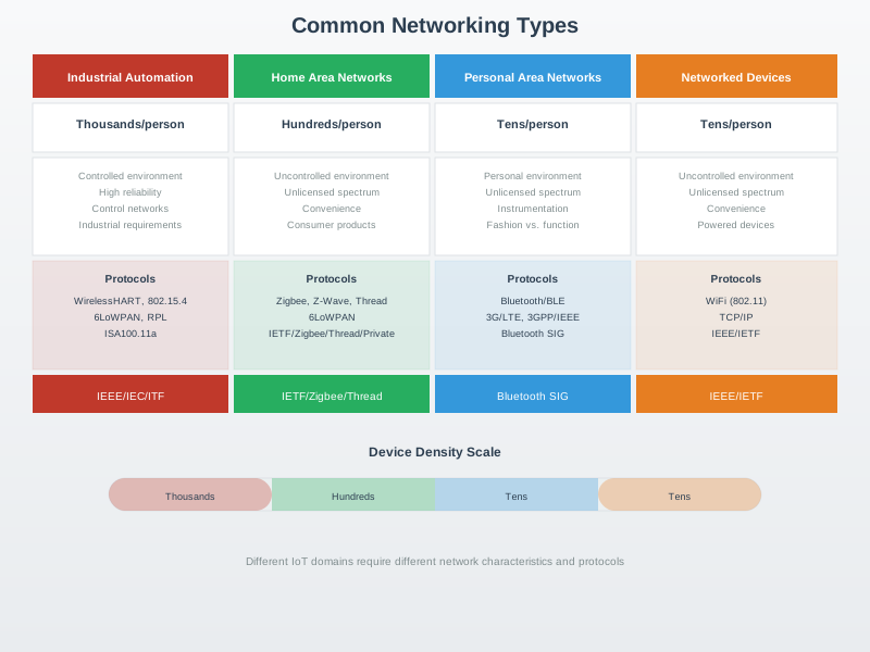
This visualization provides an overview of core networking concepts that form the foundation for understanding IoT communication systems.
Visual: Star and Mesh Topologies
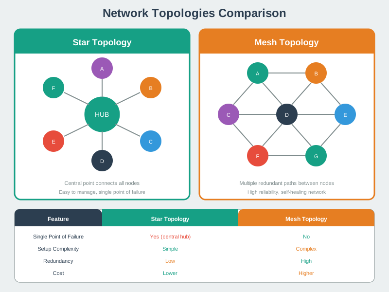
Understanding topology differences helps in selecting the right network structure for IoT deployments based on reliability, scalability, and management requirements.
Visual: Logical Network Topologies
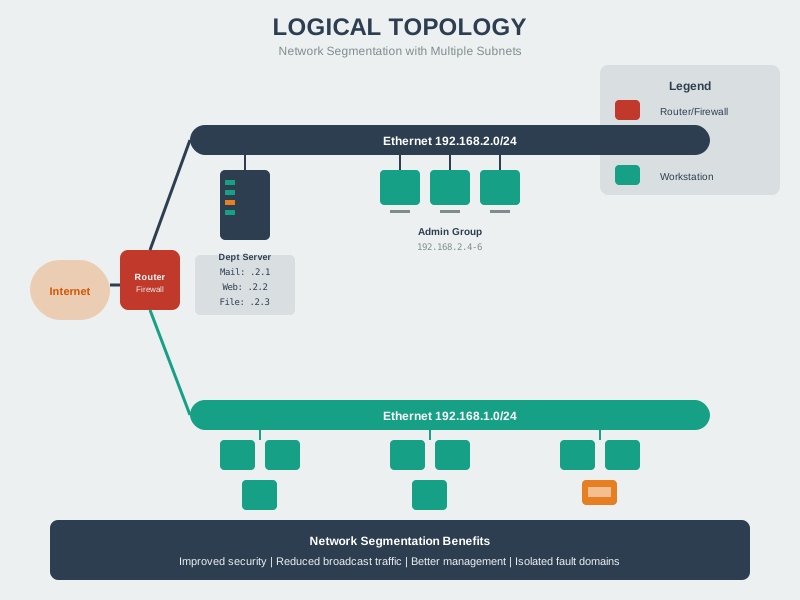
Logical topologies describe data flow patterns independent of physical cabling, helping network designers understand communication pathways.
3.14 Quick Glossary
Key Terms Reference
This glossary provides quick definitions for essential networking concepts used throughout this chapter.
| Term | Definition | Example/Context |
|---|---|---|
| IP Address | Unique numerical identifier for a device on a network | IPv4: 192.168.1.100, IPv6: 2001:db8::1 |
| MAC Address | Hardware address burned into network interface card (NIC) | 00:1A:2B:3C:4D:5E (48 bits, Layer 2) |
| Port Number | 16-bit number identifying application/service on a device | HTTP: 80, HTTPS: 443, MQTT: 1883 |
| Router | Layer 3 device that forwards packets between different networks | Home router connects LAN to internet |
| Switch | Layer 2 device that forwards frames within same network | Connects multiple devices in LAN |
| Gateway | Device connecting different network types/protocols | IoT gateway: Zigbee sensors -> Wi-Fi -> cloud |
| NAT | Network Address Translation, maps private IPs to single public IP | 192.168.1.x -> 203.0.113.42:port |
| Subnet | Logical subdivision of IP network for organization/security | Home: 192.168.1.0/24 (256 addresses) |
| Subnet Mask | Defines which portion of IP is network vs host | 255.255.255.0 = /24 (first 3 octets = network) |
| DNS | Domain Name System, converts names to IP addresses | iot.example.com -> 203.0.113.42 |
| DHCP | Dynamic Host Configuration Protocol, assigns IPs automatically | Router assigns 192.168.1.100 to new device |
| RSSI | Received Signal Strength Indicator in dBm | -50 dBm = good, -80 dBm = poor |
| TCP | Transmission Control Protocol, reliable connection-oriented transport | HTTP, MQTT, FTP use TCP (Layer 4) |
| UDP | User Datagram Protocol, unreliable connectionless transport | DNS, CoAP, streaming video use UDP |
| IPv4 | Internet Protocol version 4, 32-bit addresses (4.3 billion) | 192.168.1.1, exhausted for IoT scale |
| IPv6 | Internet Protocol version 6, 128-bit addresses (340 undecillion) | 2001:0db8:85a3::8a2e:0370:7334 |
| 6LoWPAN | IPv6 over Low-power Wireless PANs, compresses IPv6 for 802.15.4 | 40-byte IPv6 header -> 2-8 bytes |
| OSI Model | 7-layer reference model for network protocols | Physical, Data Link, Network, Transport, Session, Presentation, Application |
| TCP/IP Model | 4-layer practical internet model | Link, Internet, Transport, Application |
Network Topologies:
| Topology | Description | Pros | Cons | IoT Use Case |
|---|---|---|---|---|
| Star | All devices connect to central hub/switch | Easy to add devices, failure isolated | Hub is single point of failure | Wi-Fi access point, home network |
| Mesh | Devices interconnect with multiple paths | Redundant, self-healing | Complex routing, more power | Zigbee, Thread, WSN |
| Bus | All devices on single cable | Simple, cheap | Collisions, single point of failure | CAN bus (automotive) |
| Tree | Hierarchical star networks | Scalable, organized | Central points of failure | Industrial networks, buildings |
| Ring | Devices in closed loop | Predictable latency | Break disrupts all | Rarely used in IoT |
TCP vs UDP Comparison:
| Feature | TCP | UDP | When to Use |
|---|---|---|---|
| Connection | Connection-oriented (3-way handshake) | Connectionless | TCP: Critical data; UDP: Real-time |
| Reliability | Guaranteed delivery, retransmissions | Best-effort, no guarantees | TCP: Commands; UDP: Streaming |
| Ordering | In-order delivery | No ordering guarantee | TCP: File transfer; UDP: Gaming |
| Overhead | 20+ bytes header, state management | 8 bytes header, no state | TCP: MQTT; UDP: CoAP, DNS |
| Speed | Slower (reliability mechanisms) | Faster (no handshake) | TCP: Cloud sync; UDP: Voice |
Diagnose Wi-Fi Disconnects
Scenario: Your smart building has 50 ESP32 temperature sensors. After 3 months, 8 sensors randomly disconnect from Wi-Fi for 10-30 seconds, then reconnect. This happens 2-5 times per day.
Given Information from Diagnostics Dashboard:
- Affected sensors: RSSI fluctuates between -72 dBm and -85 dBm
- Non-affected sensors: Stable RSSI around -55 dBm to -65 dBm
- All sensors: Same firmware, same Wi-Fi credentials
- Network: 2.4 GHz Wi-Fi, Channel 6, WPA2 encryption
Step 1: Analyze RSSI Values
From the diagnostic dashboard, RSSI classifications are: - Excellent: > -50 dBm - Good: -50 to -60 dBm - Fair: -60 to -70 dBm - Poor: < -70 dBm
The affected sensors have RSSI in the “Poor” range (-72 to -85 dBm). Below -70 dBm, connection stability degrades significantly.
Step 2: Calculate Link Budget Impact
Typical ESP32 Wi-Fi specifications: - TX Power: +20 dBm - RX Sensitivity: -95 dBm (at lowest data rate) - Required margin for stable operation: 15 dB minimum
Link margin for affected sensors at -85 dBm worst case:
| Quantity | Value |
|---|---|
| Received power | -85 dBm |
| Receiver sensitivity | -95 dBm |
| Link margin | 10 dB |
| Interpretation | Below the recommended 15 dB margin, so intermittent failures are expected. |
10 dB is below the recommended 15 dB margin, explaining intermittent failures.
Step 3: Identify Root Cause
Physical inspection reveals: - Affected sensors are 25-35 meters from access point - Sensors are mounted on metal HVAC ducts (high attenuation) - Non-affected sensors are 10-20 meters away with line-of-sight
Step 4: Calculate Required Improvement
To achieve -70 dBm maximum RSSI (15 dB margin):
| Current worst RSSI | Target RSSI | Required improvement |
|---|---|---|
| -85 dBm | -70 dBm | 15 dB better signal |
Solution Options:
Option A: Add Wi-Fi extender/mesh node - Cost: $50-100 per node - Reduces path loss by 15-20 dB - Implementation time: 1 day
Option B: Relocate affected sensors - Cost: Labor only (~$200) - Improves RSSI by moving away from metal ducts - May not be feasible for some sensor locations
Option C: Increase ESP32 TX power (if using lower setting) - Cost: $0 (configuration change) - Gain: Up to 10 dB if currently limited - Trade-off: Slightly higher power consumption
Implemented Solution: Option A (mesh node) + Option C (TX power) - Added 1 mesh node covering the 8 affected sensors - Increased ESP32 TX power from +17 dBm to +20 dBm - Result: All sensors now have RSSI between -55 and -68 dBm - Link margin improved to 20-25 dB range - Zero disconnections over 30-day monitoring period
Key Lessons:
- RSSI below -70 dBm is a red flag for production deployments
- 15 dB link margin is minimum for reliable IoT Wi-Fi
- Metal surfaces (HVAC ducts, electrical panels) add 10-20 dB attenuation
- Systematic diagnostics (RSSI logging) enables data-driven troubleshooting
3.15 See Also
Related Networking Topics:
- Networking Basics: Introduction - OSI model and core concepts
- Networking Basics: Protocols and MAC - Protocol classification and selection
- Networking Basics: Hands-On Configuration - ESP32 configuration and security
Protocol Deep Dives:
- MQTT Fundamentals - Lightweight IoT messaging
- CoAP Fundamentals - Constrained application protocol
- LoRaWAN Overview - Long-range, low-power wireless
Tools and Resources:
- Wireshark - Network packet analyzer
- nmap - Network scanner
- MQTT Explorer - MQTT broker debugging
Build a Network Health Monitor
Challenge: Create a dashboard that continuously monitors your IoT network and alerts you to problems.
Requirements:
- Scan network every 5 minutes to detect new devices
- Measure RSSI, latency, and packet loss to gateway
- Send email alert if any metric exceeds threshold
- Log historical data to SD card for trend analysis
Hints:
- Use ESP32 deep sleep between scans to save power
- Store device list in SPIFFS to detect additions/removals
- Consider using MQTT to report status to cloud dashboard
- Implement exponential backoff if gateway is unreachable
Solution Approach:
| Monitor stage | Student action | Success criterion |
|---|---|---|
| Wake and connect | Bring the device online at a fixed interval. | Connection succeeds without draining the battery. |
| Measure health | Record RSSI, latency, and packet loss. | Metrics are timestamped and comparable between runs. |
| Check thresholds | Flag weak signal, high latency, or packet loss. | Alerts trigger only when a real degradation occurs. |
| Log evidence | Store recent readings locally or publish them to MQTT. | You can explain when the issue started and how long it lasted. |
| Sleep or idle | Reduce power use between checks. | Monitoring does not become the main battery drain. |
Extension Ideas:
- Add trending: Alert only if metric worsens over time
- Implement device fingerprinting: Identify device types by MAC vendor OUI
- Build web interface: Serve network map from ESP32
3.16 Practice Quizzes
Test your understanding of key networking concepts with these interactive exercises.
3.16.1 Review: Match Networking Concepts
3.16.2 Order Troubleshooting Steps
Common Pitfalls
Save Lab Configs Between Sessions
Unsaved VM snapshots or switch configurations are lost when equipment is powered off. Fix: export or save the configuration at the end of every lab session and store it in a version-controlled repository.
Avoid IP Conflicts Across Labs
Two lab topologies with the same 192.168.1.0/24 address range on the same physical switch will conflict. Fix: use different subnet ranges for simultaneous lab topologies, or use isolated VLANs or namespaces.
3. Skipping the Teardown Steps
Leaving lab VMs running, capture sessions open, or test traffic generators active interferes with subsequent labs. Fix: include explicit teardown steps at the end of every lab procedure and verify the environment is clean before starting the next exercise.
3.17 Label the Diagram
3.18 Code Challenge
3.19 Summary
Networking is the foundation of IoT. Understanding the OSI/TCP-IP models, addressing schemes, topologies, and protocols enables you to:
- Design robust IoT systems
- Troubleshoot connectivity issues
- Optimize for bandwidth and power
- Secure your devices and data
- Scale from prototypes to production
Key Takeaways:
- OSI provides framework; TCP/IP is practical implementation
- IPv6 solves address exhaustion; essential for massive IoT
- Topology choice impacts reliability, range, and complexity
- Protocol selection depends on power, bandwidth, reliability needs
- Security must be designed in, not added later
- Real-world networks are messy; design for failure
Next Steps: Now that you understand networking fundamentals, dive into specific IoT protocols (MQTT, CoAP, Bluetooth, Zigbee, LoRa) to see these concepts in action!
3.20 Additional Resources
Books:
- “Computer Networking: A Top-Down Approach” by Kurose and Ross
- “TCP/IP Illustrated” by W. Richard Stevens
Videos:
- Layered models in practice: Layered Network Models Review
- See the course-wide Video Gallery: Video Hub
Tools:
- Wireshark: Network traffic analysis
- nmap: Network scanning
- PingPlotter: Visual traceroute
- MQTT Explorer: MQTT broker monitoring
Standards:
- IEEE 802.15.4 - Low-power wireless
- RFC 791 - IPv4 Specification
- RFC 8200 - IPv6 Specification
3.21 What’s Next
You’ve completed the Networking Basics series! Continue your IoT journey with these related chapters:
- IoT Protocol Overview: IoT Protocols Overview surveys MQTT, CoAP, HTTP, and other application-layer protocols used in IoT deployments.
- Transport Layer: Transport Fundamentals dives into TCP, UDP, and IoT transport trade-offs including reliability and latency.
- Wi-Fi Standards: Wi-Fi Fundamentals covers IEEE 802.11 variants, frequency bands, and configuration choices.
- Lightweight Messaging: MQTT Fundamentals introduces publish-subscribe messaging, QoS, and broker patterns.
- Constrained Protocols: CoAP Architecture explains REST-style communication over UDP with optional DTLS security.
- Long-Range IoT: LoRaWAN Overview explores LPWAN communication for sensors that need kilometre-scale range.
Return to the Networking Basics Overview for navigation to all related chapters.