Wi-Fi feels familiar because phones and laptops use it every day, but an IoT device joins the same shared air with smaller antennas, tighter power budgets, and fewer chances for a user to fix it.
The useful design story follows association, authentication, RSSI, channel conditions, roaming, power mode, and traffic timing. A working bench connection is only the first proof.
Packet Pete
“Good signal strength is not the same claim as room on the channel — prove both before you call it delivered.”
Here Pete follows the shared air itself: what it costs to join, what it costs to stay heard, and what the record needs to show.
Key Concepts
Wi-Fi (IEEE 802.11): The dominant wireless LAN standard; multiple generations (802.11b/g/n/ac/ax) offer increasing data rates and spectrum efficiency
SSID (Service Set Identifier): The human-readable name of a Wi-Fi network, broadcast in beacon frames
Access Point (AP): The central device in a Wi-Fi star topology that all clients connect to
Channel: A designated frequency range within the 2.4 or 5 GHz bands; proper channel planning prevents inter-AP interference
OFDM (Orthogonal Frequency-Division Multiplexing): The modulation technique used by 802.11g and later; divides the channel into subcarriers to handle multipath
MIMO (Multiple-Input Multiple-Output): Using multiple antennas to send parallel data streams, increasing throughput without wider channels
WPA3: The current Wi-Fi security standard; mandatory for Wi-Fi 6 (802.11ax) certification, replacing WPA2
36.2 In 60 Seconds
Wi-Fi (IEEE 802.11) has evolved from 11 Mbps (802.11b, 1999) to multi-gigabit speeds (802.11ax/Wi-Fi 6), with two IoT-critical innovations: Wi-Fi HaLow (802.11ah) operates at sub-1 GHz for 1 km range with low power, and Wi-Fi 6 introduces OFDMA (efficient multi-device scheduling) and Target Wake Time (TWT, letting devices sleep for hours between transmissions). The 2.4 GHz band penetrates walls better but is congested, while 5 GHz is faster with less interference but shorter range.
Phoebe’s Field Notes: Where the 54 Mbps Comes From
Phoebe’s Why
Indoors, a Wi-Fi signal never arrives just once. Copies bounce off walls, floors, and furniture and reach the antenna smeared over tens to hundreds of nanoseconds – the delay spread. A single fast symbol stream at these rates would space its symbols by a comparable time, so each echo of one symbol lands on top of the next: intersymbol interference. OFDM refuses to play that game. It splits the channel into many slow parallel subcarriers, so each subcarrier’s symbol lasts microseconds – far longer than any echo – and a short guard interval in front of every symbol absorbs the smear. Echoes now corrupt only the guard, never the data.
The Split
Classic 20 MHz Wi-Fi divides the channel into 64 subcarriers:
\[\Delta f = \frac{20\ \text{MHz}}{64} = 312.5\ \text{kHz}\]
Orthogonality fixes the symbol time to the inverse of the spacing:
\[T_s = \frac{1}{\Delta f} = 3.2\ \mu\text{s}\]
A 0.8 µs guard interval – time enough for 240 m of extra echo path – brings each symbol to 4 µs. 802.11g uses 52 of the 64 subcarriers: 48 carry data, 4 are pilots. The data rate is then just bookkeeping:
\[R = \frac{b \times r \times N_{\text{data}}}{T}\]
with \(b\) bits per subcarrier, coding rate \(r\), \(N_{\text{data}} = 48\), and \(T = 4\ \mu\text{s}\).
Worked Numbers: The 54 Mbps Check
64-QAM, rate 3/4 (\(b = 6\)): \(6 \times \tfrac{3}{4} \times 48\)\(= 216\) bits per OFDM symbol; \(216 / 4\ \mu\text{s}\)\(= 54\) Mbps – exactly the table value, no rounding
SNR gates (this chapter’s modulation table): 64-QAM 3/4 needs 25 dB, QPSK 1/2 only 7 dB – the \(4.5\times\) slower link tolerates 18 dB less SNR. The \(6 \to 2\) bit step alone (\(3\times\) slower at equal coding) accounts for roughly 15 dB of that – an approximate figure, since real thresholds fold in coding gain.
This is the whole story of an access point “slowing down” at range: as received power falls (the EM-waves field notes derive why), SNR drops through gate after gate and the radio sheds bits per subcarrier – while \(\Delta f\) and \(T\) never change. One caveat: these gates assume steady, noise-like SNR. Bursty interference from neighbouring networks is not noise, which is why this chapter recommends keeping a 5–10 dB margin below the theoretical gate.
Learning Objectives
By the end of this section, you will be able to:
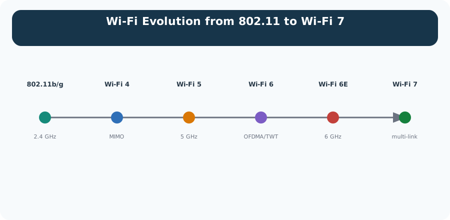
Summarize the evolution of IEEE 802.11 Wi-Fi protocols from 802.11b to Wi-Fi 7
Compare Wi-Fi standards (802.11 a/b/g/n/ac/ax) for IoT applications across speed, range, and power trade-offs
Wi-Fi is how devices connect to the internet wirelessly - like invisible cables made of radio waves! When your phone connects to your home router without a cable, that’s Wi-Fi.
Wi-Fi uses radio frequencies (like a radio station) to send data through the air. The 2.4 GHz frequency travels farther through walls but is slower and more crowded. The 5 GHz frequency is faster but doesn’t travel as far.
Term
Simple Explanation
Wi-Fi
Wireless connection using radio waves (no cables needed)
Access Point (AP)
The device that creates the Wi-Fi network (often built into router)
2.4 GHz
Radio frequency that travels far but is slow and crowded
5 GHz
Radio frequency that’s fast but doesn’t go through walls well
SSID
The name of a Wi-Fi network (like “Home_WiFi”)
RSSI
Signal strength - how strong the Wi-Fi signal is
Sensor Squad: The Wi-Fi Evolution!
“Wi-Fi keeps getting faster and smarter!” said Max the Microcontroller. “The original 802.11b from 1999 was only 11 Mbps. Now Wi-Fi 6 can do over 9 Gbps – that is nearly 900 times faster!”
“But speed is not the only improvement for IoT,” noted Sammy the Sensor. “Wi-Fi 6 has two features I love. First, OFDMA lets the router talk to many devices at the same time instead of one at a time. With hundreds of IoT devices in a smart building, that is essential.”
“Second is Target Wake Time,” added Bella the Battery with a smile. “TWT lets me negotiate a sleeping schedule with the access point. I tell it ‘wake me up in 4 hours,’ and I sleep the whole time. Before TWT, Wi-Fi devices had to wake up constantly to check for messages. TWT makes Wi-Fi actually practical for battery-powered sensors!”
Lila the LED brought up the frequency choice. “2.4 GHz goes through walls better but is crowded – every microwave, baby monitor, and Bluetooth device uses it. 5 GHz is faster and less crowded, but does not travel as far. And Wi-Fi HaLow at sub-1 GHz can reach a whole kilometer – perfect for outdoor IoT!”
36.4 IEEE 802.11 Wi-Fi Overview
Time: ~10 min | Difficulty: Intermediate | Reference: P07.C11.U03
Start with the standards history, because each generation solves a different design problem.
IEEE 802.11, commonly known as Wi-Fi, is a protocol replacing wired Ethernet for wireless communications. It uses the unlicensed radio band for data transmission.
In a Wi-Fi network, the Wireless Access Point (WAP) is responsible for translating digital signals from the wired network to radio signals, and vice versa, for communications between mobile devices in the WAP range and the Internet.
Figure 36.1: Wi-Fi evolution timeline from 802.11 Legacy to Wi-Fi 7
36.5 Wi-Fi Protocol Comparison
Standard
Year
Frequency
Max Speed
Range
IoT Suitability
802.11b
1999
2.4 GHz
11 Mbps
~100m
Low (legacy)
802.11g
2003
2.4 GHz
54 Mbps
~100m
Medium
802.11n
2009
2.4/5 GHz
600 Mbps
~200m
Good
802.11ac
2013
5 GHz
3.5 Gbps
~100m
Good (high bandwidth)
802.11ah
2016
Sub-1 GHz
347 Mbps
~1 km
Excellent (low power)
802.11ax
2021
2.4/5 GHz
9.6 Gbps
~200m
Excellent (dense)
36.6 IoT-Specific Wi-Fi Standards
The 802.11ah (Wi-Fi HaLow) and 802.11ax (Wi-Fi 6) protocols specifically address shortcomings in IoT-constrained environments.
36.6.1 802.11ah (Wi-Fi HaLow)
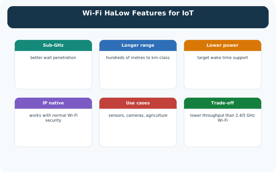
Figure 36.2: Wi-Fi HaLow features and IoT applications
Key Features:
Operates in sub-1 GHz frequency bands (better penetration through walls and obstacles)
Longer range (up to 1 km vs 100m for traditional Wi-Fi)
Lower power consumption (suitable for battery devices)
Supports large number of devices (up to 8,191 per access point)
Use cases: Smart city sensors, agricultural monitoring, industrial IoT
36.6.2 802.11ax (Wi-Fi 6)
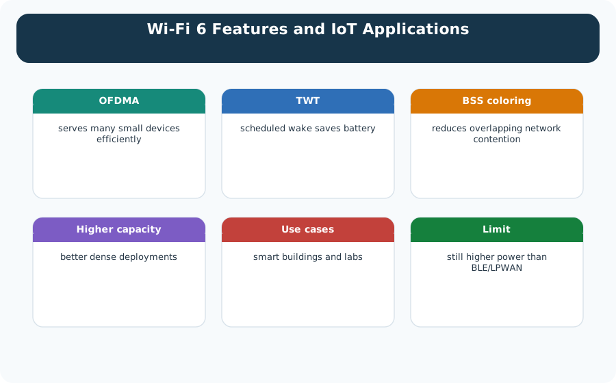
Figure 36.3: Wi-Fi 6 features and IoT applications
Key Features:
OFDMA (Orthogonal Frequency Division Multiple Access) for better multi-device handling
Target Wake Time (TWT) for power savings - devices sleep longer, wake only when needed
Higher capacity in dense environments (stadiums, offices, warehouses)
Lower latency (8ms typical vs 30ms for Wi-Fi 5)
Use cases: Smart buildings, dense sensor deployments, industrial automation
MVU: Target Wake Time (TWT)
Core Concept: TWT allows IoT devices to negotiate specific wake-up times with the access point, sleeping for extended periods rather than constantly listening for beacons - reducing power consumption by up to 90% for infrequent data transmission.
Why It Matters: Traditional Wi-Fi devices wake every 100ms to check for data, consuming significant power even when idle. TWT lets a sensor wake once per minute (or less), dramatically extending battery life from days to months.
Key Takeaway: When deploying battery-powered Wi-Fi sensors, require Wi-Fi 6 (802.11ax) support to leverage TWT. Configure appropriate wake intervals based on data reporting frequency - a sensor reporting hourly can sleep for 59 minutes between transmissions.
Checkpoint: Standards and IoT Fit
You now know:
Wi-Fi spans from 802.11b at 11 Mbps to Wi-Fi 6 at 9.6 Gbps and beyond.
HaLow trades speed for sub-1 GHz coverage, 1 km range, and up to 8,191 devices per AP.
Wi-Fi 6 adds OFDMA and TWT, which matter more to dense IoT fleets than headline speed alone.
Check Hospital Monitoring
36.7 Frequency Band Trade-offs
2.4 vs 5 GHz Wi-Fi Gateways
Option A (2.4 GHz):
Range: 100-150m indoor
Channels: 3 non-overlapping (1, 6, 11)
Interference: Crowded spectrum with Bluetooth/Zigbee/microwave
Wall penetration: -4 dB per drywall, -6 dB per concrete
Max 802.11n: 150 Mbps
Option B (5 GHz):
Range: 50-75m indoor
Channels: up to 24 non-overlapping (region-dependent)
Interference: Less interference from IoT devices
Wall penetration: -5 dB per drywall, -12 dB per concrete
Max 802.11ac: 1.3 Gbps
Decision Factors: Choose 2.4 GHz for IoT gateways requiring maximum range through walls, legacy device compatibility, or outdoor deployments. Choose 5 GHz for high-bandwidth applications (video cameras, AR/VR), dense urban environments with heavy 2.4 GHz congestion, or when gateway and devices are in the same room with minimal obstacles.
The band choice narrows the problem; modulation margin decides whether that choice remains reliable when the air gets busy.
36.8 Select Wi-Fi Modulation
Compare Wi-Fi Modulation
Scenario: Designing a Wi-Fi-connected IoT gateway that aggregates data from 50 BLE sensors. The gateway sends 10 KB data bursts to the cloud every 30 seconds. Building has 8 competing Wi-Fi networks causing channel congestion.
Given:
Data requirement: 10 KB every 30 seconds = 2.73 kbps average
Wi-Fi options: 802.11b/g/n/ac at various modulation schemes
Interference: 8 neighboring networks on overlapping channels
Power: Mains-powered (no battery constraint)
Distance to AP: 25 meters through 2 drywall partitions
Steps:
Calculate minimum required data rate:
10 KB x 1024 x 8 = 81,920 bits per burst
At 1 Mbps: ~82 ms transmission time
At 54 Mbps: ~1.5 ms transmission time
Faster = less airtime = less collision probability
Evaluate modulation schemes by robustness:
Modulation
Protocol
Max Rate
Min SNR Required
Range
BPSK 1/2
802.11a/g
6 Mbps
4 dB
Excellent
QPSK 1/2
802.11a/g
12 Mbps
7 dB
Very Good
16-QAM 1/2
802.11a/g
24 Mbps
12 dB
Good
64-QAM 3/4
802.11a/g
54 Mbps
25 dB
Fair
256-QAM 5/6
802.11ac
400+ Mbps
32 dB
Poor
Estimate link quality:
TX power: 20 dBm
Path loss: free space at 25 m is 68 dB, plus 2 interior walls at 4 dB each = 76 dB
Received power: 20 - 76 = -56 dBm
Noise floor: -95 dBm
SNR: -56 - (-95) = 39 dB (very good)
Select appropriate MCS (Modulation and Coding Scheme):
With 39 dB SNR, 256-QAM (32 dB) is theoretically possible
However, interference from 8 networks fluctuates the SNR; budget a 10 dB swing (the margin rule below)
Worst-case SNR: 39 - 10 = 29 dB
Select 64-QAM 3/4 (requires 25 dB SNR) — 4 dB of margin even in the worst case. Note how close this is: budgeting a 15 dB swing instead would push the safe choice down to 16-QAM 1/2. Margins, not peak SNR, decide the MCS.
Result: Configure the gateway for 802.11n with MCS 7 (64-QAM, 72.2 Mbps). This provides 4 dB margin above minimum SNR in worst-case interference, ensures sub-2ms burst transmission to minimize collision window, and far exceeds the 2.73 kbps requirement.
Key Insight: For IoT gateways in congested Wi-Fi environments, do NOT select the highest modulation scheme your SNR supports. Leave 5-10 dB margin for interference variability. A reliable 54 Mbps link beats an intermittent 300 Mbps link for IoT applications.
Putting Numbers to It
Wi-Fi link budget calculations determine the achievable data rate and modulation scheme based on signal strength and noise. For the IoT gateway scenario with interfering networks:
This selects 64-QAM with rate 3/4 coding (MCS 7), providing 7 dB fade margin. Using 256-QAM (requires 32 dB SNR) would leave zero margin, causing frequent link failures during interference spikes.
Transmission time for 10 KB burst at 72.2 Mbps: \[T = \frac{10 \times 8192 \text{ bits}}{72.2 \times 10^6 \text{ bps}} = 1.13 \text{ ms}\]
Sub-2ms transmission minimizes collision probability in the congested 2.4 GHz band.
Checkpoint: Band and Link Margin
You now know:
2.4 GHz offers about 100-150 m indoor reach but only three non-overlapping channels.
The gateway example starts with 20 dBm transmit power, 25 m distance, two drywall partitions, and 8 competing networks.
Margin changes the MCS decision: 64-QAM 3/4 works with a 25 dB gate only if interference still leaves enough SNR headroom.
Try It: Wi-Fi Link Budget Calculator
Adjust the parameters below to see how SNR and modulation scheme selection change for different deployment scenarios.
Show code
viewof txPower = Inputs.range([10,30], {value:20,step:1,label:"TX Power (dBm)"})viewof distance = Inputs.range([5,100], {value:25,step:5,label:"Distance to AP (m)"})viewof numWalls = Inputs.range([0,6], {value:2,step:1,label:"Drywall Partitions"})viewof numNetworks = Inputs.range([0,20], {value:8,step:1,label:"Interfering Networks"})
Objective: Use an ESP32 to scan available Wi-Fi networks and analyze their characteristics (SSID, RSSI, channel, encryption).
Hardware Required:
ESP32 development board
USB cable
Computer with Arduino IDE
The Wi-Fi range calculator above is the no-hardware version of this lab. If you have an ESP32 ready, use it to collect the same evidence: network name, RSSI, channel, and security mode.
Lab Step
What the ESP32 Scanner Collects
What to Learn From It
1
SSID for each visible network
Which networks are nearby and whether naming leaks sensitive information
2
RSSI in dBm
Whether each AP is strong enough for stable IoT connectivity
3
Channel number
Whether the site is crowded on channels 1, 6, 11, or shifted to 5 GHz
4
Encryption mode
Whether open or weak networks create security risk
5
Repeat scans in different locations
How walls, distance, and competing APs change coverage quality
Typical scan result to interpret:
SSID
RSSI
Channel
Security
Interpretation
HomeNetwork
-45 dBm
6
WPA2
Strong signal, crowded common channel
Office_WiFi
-62 dBm
11
WPA2
Usable signal, separate non-overlapping channel
Guest_Network
-58 dBm
1
WPA2
Good signal but may compete with IoT devices
IoT_Sensors
-71 dBm
6
WPA2
Marginal signal; consider closer AP or better channel plan
Analysis Tasks:
Identify channel congestion: Which channels have the most networks?
Measure signal strength: Which networks have the strongest signal (RSSI)?
Security assessment: Are there any open (unencrypted) networks?
Channel selection: If deploying a new network, which channel would you choose?
Range estimation: Based on RSSI, estimate approximate distance to access points
Once the scan gives local evidence, the case study shows how those same checks scale to thousands of devices.
36.10 Knowledge Check
Quiz: Theme Park Wearables
36.11 Wi-Fi 6 at Denver Airport
Denver International Airport (DEN) deployed Wi-Fi 6 in 2022 to support both passenger connectivity and 4,200 IoT devices across its terminal complex – making it one of the largest Wi-Fi 6 IoT deployments in a public venue.
The Challenge: The existing Wi-Fi 5 (802.11ac) network served passengers well but could not handle the growing IoT fleet: 1,800 environmental sensors (HVAC, air quality), 900 asset tracking tags (wheelchairs, carts), 800 digital signage displays, and 700 security cameras. During peak hours (6-9 AM, 4-7 PM), the access points experienced 40% channel utilization, causing sensor data delays of 500ms-2s that triggered false HVAC alarms.
Why Wi-Fi 5 Failed for IoT:
Per-AP Peak Statistic
Wi-Fi 5 Observation
Why It Hurt IoT
Connected clients
120 total: 80 passengers and 40 IoT devices
Passenger traffic competed directly with sensor traffic
Channel access method
OFDM, one device transmitting at a time
IoT packets waited behind larger client transfers
Average IoT wait time
450 ms
Sensor readings arrived too late for control decisions
Delivery success rate
87%
Missing readings created unreliable automation
False HVAC alarms
23 per day
Delayed readings looked like real system faults
Wi-Fi 6 Solution – OFDMA and TWT:
The airport deployed 340 Wi-Fi 6 access points (Cisco Catalyst 9136) with two critical configurations:
OFDMA for sensor data: Each 20 MHz channel was subdivided into 9 Resource Units (RUs), allowing 9 IoT devices to transmit simultaneously. This reduced per-device wait time from 450ms to under 50ms.
TWT for asset tracking tags: The 900 tracking tags negotiated TWT schedules – waking every 30 seconds to transmit a 12-byte location update, then sleeping. Battery life increased from 6 months (Wi-Fi 5, constant beacon listening) to 28 months (Wi-Fi 6 TWT).
Quantitative Results:
Metric
Wi-Fi 5 (Before)
Wi-Fi 6 (After)
Improvement
Sensor data latency (peak)
450 ms average
38 ms average
12x lower
Delivery success rate
87%
99.6%
+12.6%
False HVAC alarms/day
23
1-2
92% reduction
Asset tag battery life
6 months
28 months
4.7x longer
Devices per AP (peak)
120
180
50% more capacity
Annual battery replacement cost
$162,000
$34,600
$127,400 saved
Key Insight: Wi-Fi 6’s value for IoT is not about higher speeds – the sensors only need kilobits per second. The transformative features are OFDMA (simultaneous multi-device access, eliminating queuing delays) and TWT (scheduled sleep, extending battery life). For any deployment mixing high-bandwidth clients (passengers, cameras) with low-bandwidth IoT devices (sensors, tags), Wi-Fi 6 eliminates the contention that made Wi-Fi 5 unreliable for IoT at scale.
Checkpoint: Field and Case Evidence
You now know:
A scan should capture SSID, RSSI, channel, security mode, and location-to-location variation.
The hospital quiz needs Wi-Fi 6 latency near 8 ms to meet a 100 ms patient-monitoring requirement.
The airport case links 4,200 IoT devices to OFDMA, TWT, lower sensor latency, and longer asset-tag battery life.
36.12 Match Wi-Fi Standards
36.13 Wi-Fi Deployment Sequence
Common Pitfalls
Plan Wi-Fi IoT Power Use
Wi-Fi power consumption (100–200 mA active) is 10–50× higher than Zigbee or BLE. Battery-powered IoT devices on Wi-Fi may last only days. Fix: use Wi-Fi only for mains-powered IoT devices; use Zigbee, BLE, or LoRaWAN for battery-powered sensors.
Three 2.4 GHz Channels Is Not Enough
The 2.4 GHz band has only 3 non-overlapping channels (1, 6, 11). Dense AP deployments using these 3 channels cause co-channel interference. Fix: use the 5 GHz band with its 24 non-overlapping channels for dense deployments.
Use WPA3 or WPA2-Enterprise
Deploying IoT devices on an open or WPA2-Personal network exposes the entire VLAN to any device that knows the pre-shared key. Fix: isolate IoT devices on a dedicated VLAN with WPA2-Enterprise or WPA3 authentication.
Label the Diagram
Code Challenge
36.14 Wi-Fi Fit Record
Wi-Fi is not just a range or speed choice. It is a shared-airtime system where every access point, client, retry, management frame, and neighboring network competes for time on the channel.
An IoT design that says “use Wi-Fi” is incomplete until it explains how much airtime the devices need, how they authenticate, how they sleep, and how the access points will keep coverage and contention inside the deployment budget.
The design question is therefore not “does the signal reach the device?” A device can show acceptable RSSI and still lose useful service when the channel is busy, when the modulation rate falls, when hidden nodes trigger retries, or when neighboring networks reuse the same channel. Each retransmission spends more airtime before the application receives a single useful payload.
IoT makes this sharper because many devices send small messages, wake briefly, or reconnect after long sleeps. A temperature sensor, badge reader, camera, and commissioning laptop may all be “low bandwidth” in application terms, but each association, DHCP lease, TLS handshake, multicast burst, and acknowledgment still consumes channel time. The Wi-Fi decision must include the access point, channel width, band, security method, client power behavior, and backhaul path as one service contract.
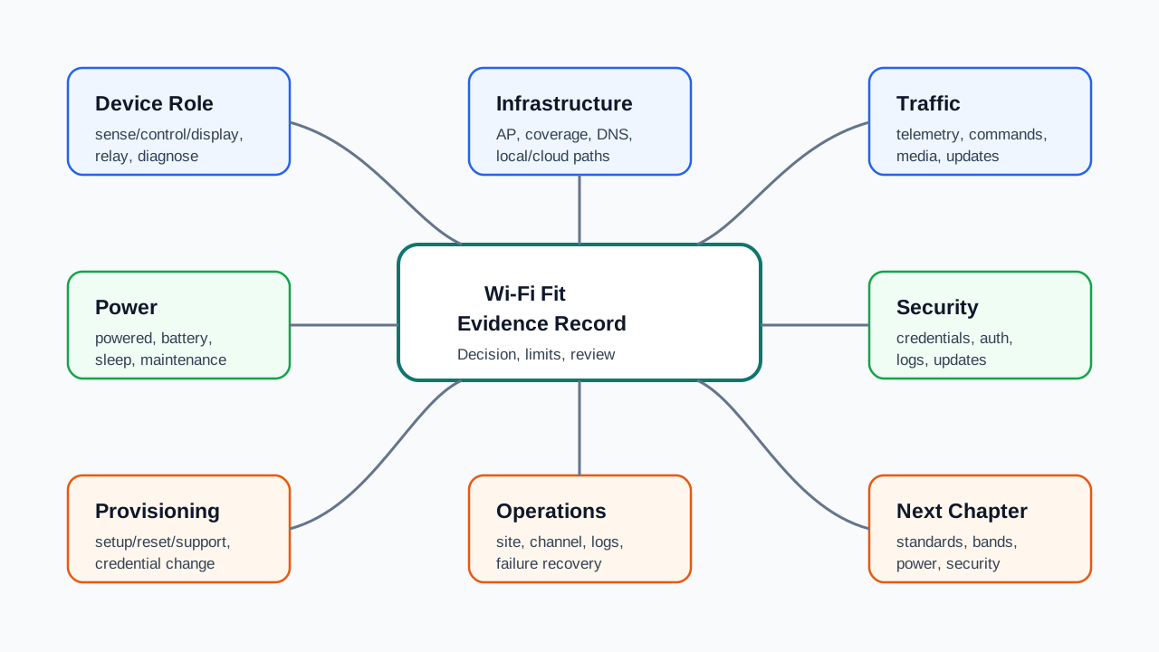
A good fit record separates coverage, capacity, and operations evidence. Coverage proves the client can hear and be heard. Capacity proves the channel has enough airtime during busy periods. Operations evidence proves the design can survive firmware updates, credential rotation, AP replacement, and site changes without forcing a truck roll for every sleeping device.
Pete’s Delivery Slip
Address: a device can show acceptable signal strength and still lose service when the channel is busy.
Route: association, DHCP lease, TLS handshake, and every acknowledgment still spend airtime, even for a “low-bandwidth” sensor.
Receipt: coverage proves the client can be heard – capacity proves the channel has time to hear it back.
Figure 36.4: Wi-Fi fit evidence record linking device role, infrastructure, traffic, power, security, provisioning, operations, and next review areas.
Fit question
What to verify
Typical failure mode
Coverage
RSSI, SNR, antenna orientation, wall loss, and roaming boundaries
Device can associate but falls to low MCS rates or retries heavily
Capacity
Device count, traffic shape, modulation rate, retries, and channel reuse
“Low-bandwidth” devices still stall because management traffic and retries consume airtime
Power
Listen interval, DTIM, Target Wake Time, and reconnect behavior
Battery devices spend energy waiting, rejoining, or retrying instead of sleeping
Design signal
Choose Wi-Fi when the application needs IP reachability and moderate to high throughput, and when the site can support measured airtime, managed channels, and appropriate security.
36.15 Wi-Fi Capacity Record
A useful Wi-Fi record turns radio assumptions into field checks. It should show what each device sends, how often it wakes, which access point serves it, what minimum signal quality is acceptable, and what happens when the channel is busy.
Build the record from measured evidence, not vendor coverage claims. For each device class, record the band, channel width, SSID, authentication method, VLAN, expected packet size and cadence, peak burst behavior, firmware-update path, and battery sleep pattern. Then attach site evidence: AP placement, survey readings at installed height, noise floor, channel utilization, retry percentage, client MCS rates, roaming results, and backhaul utilization during the busiest period you can reproduce.
The record should also document what the design will not support. A 2.4 GHz-only sensor may be acceptable for low-rate telemetry, but it competes with legacy clients and neighboring networks. A high-resolution camera may need 5 GHz or 6 GHz capacity, but it may lose range faster through walls. A battery device may support long sleep intervals, but failed joins, certificate renewal, or captive provisioning can dominate energy use if the network path is unreliable.
Pete’s Delivery Slip
Address: a useful record names what each device class sends, how often it wakes, and which access point serves it.
Route: overlapping channels create contention even when each access point looks healthy on its own.
Receipt: measured survey and retry-rate evidence beats a vendor coverage claim every time.
Record field
Example value
Why it matters
Evidence to keep
Coverage target
-67 dBm RSSI, 25 dB SNR at sensor mount points
Weak signal forces lower modulation, longer airtime, and more retries
Survey heat map and measured client RSSI
Channel plan
2.4 GHz channels 1/6/11 for legacy sensors; 5 GHz for cameras
Overlapping channels create contention even when each AP looks healthy
Small packets still consume contention overhead, acknowledgments, and wake time
Airtime estimate and packet capture sample
Security and roaming
WPA2-Enterprise or WPA3, IoT VLAN, sticky-client threshold tested
Authentication delay and roaming behavior can break mobile or sleep-heavy devices
Auth logs, VLAN map, roaming test notes
Deployment moment
Checks to perform
Before install
Measure noise floor, interference, AP placement, antenna pattern, and expected client density for each coverage zone.
During commissioning
Verify association time, DHCP or static addressing, TLS handshake, retry rate, roaming path, and actual upload latency.
During operations
Watch airtime utilization, channel changes, retry percentage, deauth events, client MCS rates, and battery drain after firmware updates.
Escalation trigger
If average RSSI is acceptable but retry rate or latency is high, treat the issue as capacity, interference, or hidden-node contention instead of adding transmit power first.
The fit record turns selection into operations: it says what to measure after installation, not just what standard to buy.
36.16 OFDMA and TWT Schedule Contention
Wi-Fi 6 improves dense IoT service by giving the access point better tools for scheduling. OFDMA divides a channel into resource units so multiple clients can send in a coordinated transmission window. Target Wake Time lets clients agree on sleep and wake schedules instead of listening constantly.
Those tools do not remove the shared medium. Beacons, probe traffic, acknowledgments, retransmissions, hidden nodes, low modulation rates, and neighboring networks still consume airtime. A slow or distant device can reduce usable capacity because each frame takes longer to deliver.
Classic Wi-Fi access is contention-based. A station listens before transmitting, waits through interframe spacing, chooses a random backoff when the medium is busy, and expects an acknowledgment for unicast frames. If the acknowledgment is missed, the frame is retried at additional airtime cost. This is why retry rate and airtime utilization often explain user-visible stalls better than headline PHY rate.
OFDMA changes the scheduling granularity, not the need for planning. In Wi-Fi 6, the access point can divide a channel into resource units and coordinate multiple clients during a transmission opportunity, including trigger-based uplink traffic when clients and the AP support it. That helps dense small-packet workloads, but it depends on compatible clients, firmware behavior, AP scheduler policy, channel conditions, and whether the traffic arrives in patterns the scheduler can combine.
Target Wake Time is also a contract. The AP and client agree when the client can wake for service, so the device spends less energy listening between events. It works best when sensor deadlines, AP buffering, beacon/DTIM behavior, IP lease timing, and security renewal all fit the wake plan. If a device wakes outside its agreed window, roams unexpectedly, or must reauthenticate after sleep, the power saving can disappear into repeated join and retry work.
Mechanism
Where it helps
What still limits it
OFDMA
Many clients have small packets ready at similar times and the AP can coordinate them efficiently
Client compatibility, AP scheduler policy, channel quality, and traffic burst alignment
TWT
Battery clients can sleep between scheduled service windows
Sensor deadlines, buffering limits, beacon/DTIM behavior, IP lease timing, and security renewal
Retry control
Airtime stays available for useful payloads instead of repeated failed frames
Interference, weak signal, hidden nodes, motion, and low modulation fallback
Knowledge Check: Wi-Fi Airtime Capacity
Checkpoint: Operations Contract
You now know:
A fit record separates coverage, capacity, power, security, provisioning, and operations evidence.
Good RSSI is not enough; retry rate, airtime utilization, MCS fallback, roaming, and hidden-node behavior can still break service.
OFDMA and TWT help only when clients, AP scheduling, buffering, wake timing, and traffic bursts line up.
36.17 Summary
Wi-Fi provides high-bandwidth wireless connectivity for IoT, with recent standards specifically designed for IoT applications.
Key Takeaways
Wi-Fi for IoT:
802.11n: General IoT where dual-band support and MIMO are enough.
802.11ac: Video and other high-bandwidth devices that benefit from fast 5 GHz links.
802.11ah (Wi-Fi HaLow): Long-range sensors that need sub-1 GHz coverage and lower power.
802.11ax (Wi-Fi 6): Dense deployments where OFDMA and Target Wake Time improve capacity and battery life.
IoT-Specific Features:
Wi-Fi HaLow: Sub-1 GHz for 1km range, 8,191 devices/AP, battery-friendly
Wi-Fi 6: OFDMA for efficient multi-device, TWT for power savings, 8ms latency
Selection Criteria:
Range: HaLow for 1km, traditional for 100m
Power: Wi-Fi 6 TWT or HaLow for battery devices
Bandwidth: Wi-Fi 5/6 for video, HaLow for sensors
Density: Wi-Fi 6 OFDMA for many devices
Best Practices:
Use Wi-Fi 6 for new IoT deployments (TWT, OFDMA)
Consider HaLow for outdoor/long-range sensors
Design for 5-10 dB SNR margin in congested environments
Use 5 GHz where possible to avoid 2.4 GHz congestion
Plan AP density based on device count and bandwidth needs