15  WSN Duty Cycle Worked Examples

Keywords

duty cycle worked examples, average current, sensor node sleep schedule, wake overhead, current ledger, retest trigger

15.1 Start With the Field Story

Treat each duty-cycle example as a small energy ledger. List the states, attach a current draw and time share to each one, include wake and communication overhead, then ask whether the resulting average current matches the lifetime claim.

15.2 In 60 Seconds

Duty-cycle examples are useful when each calculation is tied to an evidence record. A reviewable example lists the states, current draw, active interval, cycle length, omitted overhead, average-current result, and retest trigger.

This chapter uses supplied exercise values only. The goal is not to promise an operating interval for a particular node. The goal is to show how to check a duty-cycle claim, find missing states, and write a bounded decision.

Phoebe’s Field Notes: The mA Ledger Hides A Volt And A Band Choice

Phoebe’s Why

Every ledger in this chapter sums current times time and calls the result “the answer,” but a mA·ms total is charge, not energy, and charge alone cannot say whether the node survives. Charge only becomes energy once it is multiplied by a voltage – and that voltage is not the constant number on the cell’s label. Under a current pulse, a battery’s own internal resistance steals some of the voltage before it reaches the radio, so the biggest single term in any ledger (the transmit burst) is exactly the moment the supply is weakest. The nameplate capacity is not usable either: shelf self-discharge, cold-temperature derating, and the cutoff voltage a regulator actually needs all strand charge the ledger never gets to spend. And the transmit term’s duration – the 40 ms this chapter keeps reusing – is itself a frequency-band choice: a slower sub-GHz PHY needs far longer on air to move the same bits than a 2.4 GHz PHY does, so choosing the band changes the ledger before a single milliamp is measured.

The Derivation

Charge is current integrated over time; energy also needs the voltage it moved through:

\[Q = \int I\,dt \ (\mathrm{mAh}), \qquad E\,(\mathrm{Wh}) \approx V \times Q\,(\mathrm{Ah})\]

A cell sags under load by its internal resistance:

\[V_{term} = V_{oc} - I\,R_{int}\]

Usable charge is nameplate charge reduced by every derating factor stacked together:

\[Q_{usable} = Q_{nameplate}\times(1-f_{self})\times(1-f_{temp})\times(1-f_{cutoff})\]

A transmit burst’s duration is payload size divided by the band’s bit rate, which sets that state’s contribution to the ledger:

\[t_{tx} = \frac{\text{payload bits}}{\text{bit rate}}, \qquad \text{charge}_{tx} = I_{tx}\times t_{tx}\]

Worked Numbers: This Chapter’s Own 24 mA, 40 ms Burst

• Sag during Example 1’s transmit state (catalog-typical CR2032, \(V_{oc}=3.0\) V, \(R_{int}=20\ \Omega\) moderately depleted): \(\Delta V = 0.024\times20\) \(= 0.480\) V \(\to\) terminal falls to \(2.52\) V during the \(24\) mA burst – only \(0.12\) V above a catalog-typical \(2.4\) V brownout threshold
• Usable capacity (catalog-typical CR2032, \(225\) mAh nameplate; \(2\%\) two-year self-discharge, \(15\%\) cold derate, \(16\%\) cutoff headroom): \(225\times0.98\times0.85\times0.84\) \(= 157\) mAh usable
• Lifetime check against this chapter’s own \(0.213\) mA average: \(157/0.213\) \(= 739\) h \(\approx 30.8\) days – a bounded decision the mA·ms ledger alone cannot produce without the voltage and derating steps above
• Band choice changes the transmit term: this chapter’s \(40\) ms burst at \(24\) mA implies a payload of about \(160\) bits (\(20\) bytes) moved at roughly \(160/0.040\) \(= 4{,}000\) bit/s, a sub-GHz-class rate. The same \(160\) bits at a \(250\) kbit/s 2.4 GHz PHY take \(160/250{,}000\) \(= 0.640\) ms, cutting that state’s charge from \(40\times24=960\) mA·ms to \(0.640\times24\) \(= 15.4\) mA·ms – a \(98.4\%\) drop in the single largest term of the ledger, entirely from the band’s bit rate, not the current

15.3 Learning Objectives

By the end of this chapter, you will be able to:

• Build a state ledger for a duty-cycled sensor node.
• Compute average current from active, wake, transmit, listen, and sleep states.
• Solve for a cycle length from a current budget.
• Compare a simple calculation with a measured trace and explain the gap.
• Record validation evidence and retest triggers for duty-cycle examples.

15.4 Quick Check: Duty Cycle Worked Examples

15.5 Minimum Viable Understanding

1. Duty cycle is an active fraction, but average current depends on every state in the cycle.
2. Sleep current is small per instant but can dominate a long cycle.
3. Wake, listen, guard, and transmit states should not be hidden inside a single active number.
4. A current budget can be used to solve for the longest acceptable cycle length.
5. Weighted mode examples must state how much of the record is spent in each mode.
6. A calculation is not accepted until the record states what was measured, assumed, and excluded.

15.6 Prerequisites

• WSN Energy Duty Cycling: active fraction, sleep states, average-current basics, and schedule evidence.
• WSN Energy Management: why battery, current, latency, and measurement records belong in the same design review.
• Topology Management Techniques: follow-on review of topology policies.

15.7 Review Pattern

Each worked example should produce a short review record:

• Question: what claim is being checked?
• State ledger: which states occur in one cycle?
• Inputs: current draw, active interval, cycle length, and units.
• Calculation: current-time sum divided by the full cycle length.
• Evidence: trace, log, or inspection that supports the inputs.
• Decision: accept, revise, or retest.
• Retest trigger: the change that makes the calculation stale.

Figure 15.1: Duty-cycle worked example state ledger (Example 1): sensing, transmit, wake, and sleep terms sum to 2,128.05 mA·ms, divided by the 10,000 ms cycle for a 0.213 mA average.

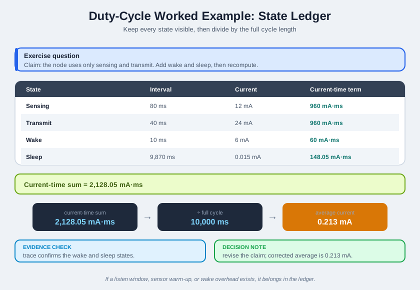
Use Figure 15.1 as the structure for each example. The important move is to keep omitted states visible. If a radio listen window, sensor warm-up, or wake overhead is present, it belongs in the ledger.

Concrete example context: treat each exercise as a review of a battery-powered status node, such as a leak detector or soil-moisture node, before its schedule is accepted for a field trial. The arithmetic is useful only because the ledger explains what the node actually does during wake, sense, listen, transmit, and sleep states.

15.8 Example 1: Expand A Simple Cycle

Question

A learner claims that a node uses only its sensing and transmit states during a repeating cycle. Check the average-current result after adding wake and sleep states.

Given exercise record

• Sensing state: 80 ms at 12 mA.
• Transmit state: 40 ms at 24 mA.
• Wake overhead: 10 ms at 6 mA.
• Sleep state: remaining interval at 0.015 mA.
• Full cycle length: 10,000 ms.

Step 1: compute the known current-time terms

sensing  = 80 ms  x 12 mA  = 960 mA*ms
transmit = 40 ms  x 24 mA  = 960 mA*ms
wake     = 10 ms  x 6 mA   = 60 mA*ms

Step 2: compute the sleep interval

sleep interval = 10,000 ms - 80 ms - 40 ms - 10 ms
sleep interval = 9,870 ms
sleep term     = 9,870 ms x 0.015 mA = 148.05 mA*ms

Step 3: divide by the full cycle length

current-time sum = 960 + 960 + 60 + 148.05
current-time sum = 2,128.05 mA*ms
average current  = 2,128.05 / 10,000
average current  = 0.213 mA

Decision

Revise the original claim if it omitted wake or sleep states. The corrected average current for this exercise record is 0.213 mA.

Retest trigger

Repeat the review if any state interval, current draw, cycle length, or radio behavior changes.

15.9 Example 2: Solve For The Cycle Length

Question

A review record gives the maximum average current as 0.080 mA. Determine the cycle length that keeps the example at or below that budget.

Given exercise record

• Wake state: 15 ms at 8 mA.
• Sensing state: 120 ms at 10 mA.
• Transmit state: 60 ms at 28 mA.
• Sleep current: 0.012 mA.
• Maximum average current: 0.080 mA.

Step 1: compute active current-time sum

wake     = 15 ms  x 8 mA  = 120 mA*ms
sensing  = 120 ms x 10 mA = 1,200 mA*ms
transmit = 60 ms  x 28 mA = 1,680 mA*ms
active current-time sum = 3,000 mA*ms
active interval = 195 ms

Step 2: solve for cycle length

Let T be the full cycle length in milliseconds.

0.080 = (3,000 + 0.012 x (T - 195)) / T
0.080T = 3,000 + 0.012T - 2.34
0.068T = 2,997.66
T = 44,083 ms

Step 3: interpret the answer

The cycle length must be at least about 44.1 s for the supplied values to meet the current budget. A shorter cycle can still work if another state is reduced, but that new design needs its own record.

Decision

Accept the schedule only if the implementation actually uses a cycle length at or above the computed value and the trace confirms the listed states.

Retest trigger

Repeat the review if the current budget, active interval, transmit interval, or sleep current changes.

15.10 Example 3: Weighted Modes

Question

A node has three operating modes during an observation record. Compute the weighted average current and decide whether the record supports the current budget.

Given exercise record

• Baseline mode: fraction 0.80, average current 0.050 mA.
• Watch mode: fraction 0.15, average current 0.200 mA.
• Event mode: fraction 0.05, average current 1.000 mA.
• Current budget: 0.150 mA.

Step 1: multiply each mode by its fraction

baseline contribution = 0.80 x 0.050 mA = 0.040 mA
watch contribution    = 0.15 x 0.200 mA = 0.030 mA
event contribution    = 0.05 x 1.000 mA = 0.050 mA

Step 2: add the contributions

weighted average current = 0.040 + 0.030 + 0.050
weighted average current = 0.120 mA

Decision

Accept the calculation for the supplied observation record because 0.120 mA is below the 0.150 mA budget. The decision is bounded to the stated mode fractions.

Retest trigger

Repeat the review if event mode becomes more common, if any mode current changes, or if the mode classification rule changes.

15.11 Example 4: Explain A Measurement Gap

Question

A simple ledger predicts 0.210 mA, but a measured trace shows 0.300 mA. Find a plausible missing state before changing the schedule.

Given exercise record

• Simple ledger result: 0.210 mA.
• Measured trace result: 0.300 mA.
• Full cycle length: 10,000 ms.
• Trace inspection finds a guard-listen state: 60 ms at 15 mA.

Step 1: compute the missing guard-listen contribution

guard-listen term = 60 ms x 15 mA = 900 mA*ms
guard-listen average contribution = 900 / 10,000
guard-listen average contribution = 0.090 mA

Step 2: add it to the simple ledger

corrected average current = 0.210 mA + 0.090 mA
corrected average current = 0.300 mA

Decision

The measured trace is consistent with the missing guard-listen state. Revise the ledger rather than treating the measurement as a fault.

Retest trigger

Repeat the review if guard-listen length, synchronization policy, radio state, or cycle length changes.

Figure 15.2: Duty-cycle worked example review loop: six stages with the Example 4 guard-listen arithmetic that closes a 0.210-to-0.300 mA gap.

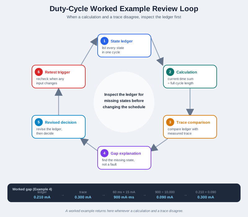
Use Figure 15.2 when a calculation and trace disagree. The first response should be to inspect the ledger for missing states before changing the schedule.

15.12 Review Checklist

Before accepting a duty-cycle worked example, check:

• Is the question stated?
• Are all state intervals listed with units?
• Are current values recorded in a consistent unit?
• Does the calculation divide by the full cycle length?
• Are wake, listen, guard, and transmit states included when present?
• Is the evidence source named?
• Is the decision bounded to the supplied record?
• Is the retest trigger explicit?

15.13 Knowledge Check

15.14 Matching Quiz

15.15 Ordering Quiz

15.16 Duty Cycle Becomes A Battery-Life Claim

Duty-cycle arithmetic is useful only when it stays tied to the review record. The short chain is: a duty cycle sets an average current, average current divided into battery capacity gives lifetime, and the evidence record states which states were included or excluded. A node that sleeps 99% of the time may move from days to years of operation, but only if the ledger includes wake, listen, transmit, and sleep behavior instead of just the headline active fraction.

Figure 15.3: Duty cycle impact on battery life: for a 2000 mAh battery, always-on versus a 1% duty cycle changes the average current and extends lifetime from days to years.

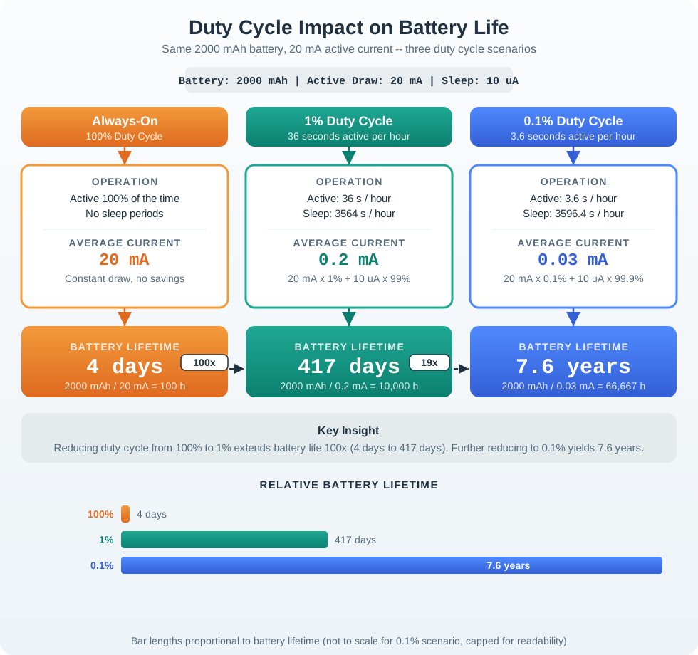
Read the ledger left to right: name the state, multiply current by time, add every contribution, and divide by the full period. The formula is reviewable only when the state rows are visible.

The same average-current ledger can support an operating-life estimate, but the estimate inherits every assumption in the ledger. A field note that says “2% duty cycle” is not enough if the node also wakes an oscillator, waits through a guard interval, listens for a parent, retries a transmit, or leaves a sensor rail biased after the sample.

For a novice, the easiest mental model is a phone that spends most of the day with its screen off. The screen-off time helps, but the phone still drains if background radios, sensors, or apps keep running. A sensor node is the same kind of accounting problem at smaller currents. The ledger is not extra paperwork; it is the place where hidden always-on behavior becomes visible. If the ledger says “sleep” but a pull-up, regulator, or sensor bias remains on, the battery-life claim is already optimistic.

That is why the worked examples in the body stop at bounded decisions instead of announcing a universal lifetime. Each arithmetic answer is a claim about one record, one set of states, and one evidence source. When the hardware or schedule changes, the record must be rerun before the lifetime story is reused.

15.17 Average Current To Lifetime

Average current blends the active and sleep states weighted by duty cycle D:

I_avg = D x I_active + (1 - D) x I_sleep

Then lifetime = battery capacity / I_avg. Take a node with I_active = 20 mA, I_sleep = 5 uA, a 2000 mAh battery, and a 1% duty cycle:

Step	Value
Active contribution	0.01 x 20 mA = 0.20 mA
Sleep contribution	0.99 x 0.005 mA ~= 0.005 mA
Average current	~= 0.205 mA
Lifetime	2000 mAh / 0.205 mA ~= 9750 h ~= 1.1 years

Two practical details keep this calculation honest. First, the units must agree: battery capacity in mAh divided by average current in mA gives hours, not seconds or cycles. Second, the capacity number is not a perfect fuel tank. Temperature, battery chemistry, regulator efficiency, cutoff voltage, pulse current, and ageing can reduce usable capacity, so a production record should treat the arithmetic lifetime as an upper-bound estimate unless the battery test supports it.

The calculation also tells the practitioner which measurement to improve next. If active current dominates, shortening transmit time or reducing radio current can move the result. If sleep current dominates, a better active routine may barely matter; the useful work is finding leakage, sleep-mode mistakes, or always-on peripherals. A reviewable example names that controlling term so the next lab measures the right state instead of repeating the same average-current calculation.

The same node at 100% duty draws 20 mA and lasts about 100 hours, roughly four days. Dropping to a 1% duty cycle multiplies lifetime by nearly 100x, but the decision is still bounded to this battery, this active current, this sleep current, and this duty cycle. If any of those terms changes, the lifetime estimate needs a new record.

Practitioner check: when a worked example solves for cycle length, state the result as a constraint, not a promise. “At least 44.1 s for this ledger” is reviewable; “the node lasts long enough” is not.

15.18 Sleep Current Sets The Floor

Look again at the numbers as the duty cycle keeps falling. At 1% duty the active term (0.20 mA) still dominates the sleep term (0.005 mA). At 0.01% duty the active contribution drops to about 0.002 mA, below the 0.005 mA sleep current. Beyond that point, cutting the duty cycle further barely helps because the node’s lifetime is set by what it draws while asleep. Sleep current becomes the floor on average current, and therefore the ceiling on battery life.

This reframes low-power engineering. Once your duty cycle is very low, the payoff moves from “wake less often” to “sleep more deeply”: a microcontroller sleep mode of 5 uA versus 50 uA changes the lifetime floor by 10x at those duty cycles, while shaving the active time does almost nothing. It also explains why designers scrutinize leakage, brown-out circuitry, and always-on peripherals: at aggressive duty cycles, the microamps you cannot switch off are the whole game. The worked numbers are not just a lifetime estimate; they tell you which parameter to optimize next.

Worked example: the crossover point. The active term equals the sleep term when D x Iactive = (1 - D) x Isleep. With Iactive = 20 mA and Isleep = 0.005 mA, the crossover is approximately D = 0.005 / (20 + 0.005) = 0.00025, or 0.025%. Above that duty cycle, the active burst is still the larger contributor. Below it, sleep current dominates. A 0.01% duty cycle is below the crossover, so a designer should first audit leakage, sleep-mode selection, regulator quiescent current, pull-up paths, and sensors left biased during sleep.

The floor also explains why measurement traces can disagree with tidy ledgers. A meter set to average current may hide a short 24 mA transmit pulse, while a slow logging interval may miss a 6 mA wake ramp. Conversely, an unexpected 10 uA leakage path can double a nominal 5 uA sleep floor and erase the benefit of rare wakeups. Under the hood, duty-cycle examples are not just algebra: they are a model of where current flows in time, which instrument can see it, and which omitted state would change the final decision.

15.19 Summary

Duty-cycle worked examples should preserve the evidence behind the arithmetic. A complete review record states the question, lists every state, computes current-time terms, divides by the full cycle length, compares the result with evidence or a current budget, and records a retest trigger. Missing wake, listen, guard, or transmit states are common reasons a simple calculation disagrees with a measured trace.

15.20 Key Takeaway

Duty-cycle worked examples should show the energy, latency, sensing, communication, and failure assumptions behind each schedule.

15.21 Concept Relationships

• Duty Cycle Fundamentals define active fraction and average-current vocabulary.
• State ledgers make each operating state visible.
• Weighted modes connect adaptive schedules to observed mode fractions.
• Trace comparison separates missing states from measurement faults.
• Retest triggers keep calculations tied to the current design record.

15.22 What’s Next

Previous: WSN Duty Cycling

Next: WSN Deployment Sizing

Use WSN Duty Cycling to review sleep/wake scheduling and measurement evidence. Continue to WSN Deployment Sizing to connect energy records with field deployment constraints.