flowchart LR
  A["Timestamp and value stream"] --> B["Delta-of-delta timestamps"]
  A --> C["Delta or XOR values"]
  B --> D["Small codes and bit runs"]
  C --> D
  D --> E["Compressed block"]
  E --> F["Exact reconstruction"]
42 Time-Series Compression Audit Limits
analytics-ml
edge
acq
time
42.1 Start With the Story
Picture an IoT team using the ideas in Time-Series Compression Audit Limits during a live operations review. A device has produced messy evidence, an analytic step is about to change an alert or control decision, and someone has to explain why the result should be trusted.
Read this page as that path from sensor evidence to accountable action. Start with what the system observes, keep the model or data treatment visible, and finish with the check that would convince an operator, maintainer, or auditor to act.
42.2 Learning Objectives
After this page, you should be able to:
- Explain why regular timestamps and slowly changing values make sensor streams highly compressible.
- Separate delta, delta-of-delta, and Gorilla-style XOR encoding roles in time-series blocks.
- Decide when lossless compression is required and when lossy reductions are acceptable.
- Record compression metadata so cloud analytics can judge audit-grade, trend-grade, or exploratory evidence.
42.3 Why Compression Follows Sampling
Edge Sampling and Compression teaches the main sampling, aggregation, FFT, semantic extraction, and edge algorithm-selection workflow. This page narrows in on the deeper storage boundary: how a stream can shrink without changing facts, and how to prove which facts were preserved.
Use it when an edge node, gateway, or time-series store must reduce bytes while still supporting incident review, compliance, trend dashboards, or machine-learning features with clear fidelity guarantees.
42.4 Compress Similar Samples
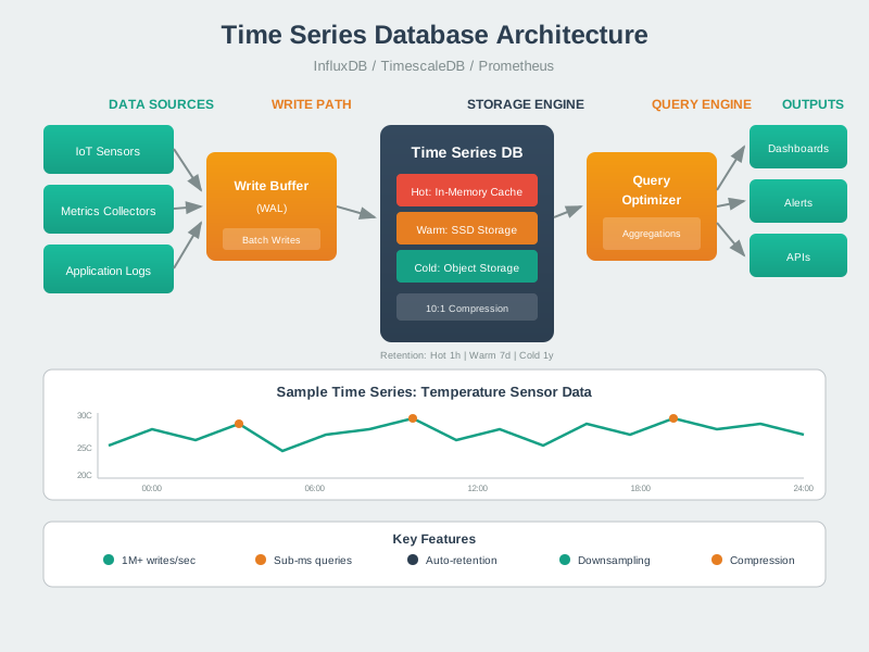
A sensor emits a relentless stream of timestamped values, and in most streams each value is very close to the one before it, arriving at a very regular interval. Storing or transmitting every full value and full timestamp wastes space on redundancy. Time-series compression exploits exactly that redundancy to store the same data in a fraction of the space – and, crucially, losslessly.
Two ideas carry most of the gain: encode differences rather than absolute values (they are small when the signal changes slowly), and exploit the bit-level similarity of consecutive floating-point numbers. These power production time-series databases and cut the amount of data an edge node must ship.
Intuition: instead of writing “20.01, 20.02, 20.01, 20.03” in full, write the first value and then “+0.01, -0.01, +0.02”. The changes are tiny, so they need far fewer bits than the full numbers.
Worked example: a refrigerated-truck sensor reports temperature every second. The raw log stores a 64-bit timestamp and a 64-bit floating value for each point, so one hour is 3,600 points times 16 bytes, or 57,600 bytes before protocol overhead. If the timestamp interval is almost always one second, delta-of-delta mostly records zero. If the value moves from 3.01 C to 3.02 C to 3.02 C, value deltas or XORs are also small. The compressor keeps the same facts, but it stops paying full width for repeated structure during radio upload.
The boundary is fidelity: compression is acceptable only when the receiver can still answer the same question. A maintenance alarm, an audit log, and a trend dashboard may all use the same source stream, but each needs a different guarantee about what was preserved.
42.4.1 Overview Knowledge Check
42.5 Practitioner: Delta Encoding and Gorilla
Delta encoding: store (value - previous_value); small when slow-changing
Delta-of-delta (timestamps): regular intervals -> the change in interval
                is ~0, encodable in a single bit most of the time
Gorilla (values): XOR each float with the previous one; similar floats
                share most bits, so the XOR is mostly zeros -> store only
                the meaningful middle bits plus their position
Worked example: Gorilla’s real-world result
A raw point = (64-bit timestamp, 64-bit double) = 16 bytes.

Facebook's Gorilla, on real production monitoring data:
  - delta-of-delta on timestamps (mostly regular) -> ~1 bit each
  - XOR compression on the doubles (mostly similar) -> few bits each
  Average: about 1.37 bytes per point.

That is roughly a 12x reduction from 16 bytes -- lossless,
so every value reconstructs exactly.
Splitting the work by column is deliberate: timestamps compress best with delta-of-delta (they are almost perfectly regular), while values compress best with XOR (they are numerically similar but not linearly spaced). Each column gets the scheme that fits it.
Worked example continuation: if a gateway receives 10,000 points from one sensor, a row layout repeats timestamp and value metadata for each record. A columnar block instead stores a timestamp column, a value column, and a small header that says which compression method each column used. On readback, the decompressor expands timestamp intervals, applies value XOR or deltas in order, and reconstructs the original point sequence. The application still sees ordinary timestamp-value pairs, but the radio and flash never had to carry the repeated full-width representation.
For a practitioner, the check is simple: compress a representative block, decompress it, and compare every timestamp and value against the original before measuring the byte savings. Repeat that check on quiet periods, noisy transitions, and missing-sample gaps.
Also record the compression parameters beside the block: sample period, time base, value type, scale factor, algorithm, version, and whether any samples were dropped before compression. Without that metadata, a future decoder may recover numbers correctly but attach the wrong meaning to them.
42.5.1 Practitioner Knowledge Check
42.6 Lossless, Lossy, and Edge Payoff
Compression decisions sit on two axes: reconstruction and decision value. Lossless methods must return the exact original sequence, so they are appropriate for billing, compliance, incident review, and any record where a later investigator may ask what the sensor actually reported. Delta, delta-of-delta, run-length, and Gorilla-style XOR encoders are in this family. They exploit regularity, but they do not change the facts.
Lossy methods intentionally throw away detail. Window aggregation, downsampling, piecewise-linear approximation, FFT peak extraction, and event extraction can reduce a stream far more than lossless compression, but the discarded detail is gone. That is acceptable only when the downstream question is known. A trend dashboard may need hourly min, max, and mean; a vibration diagnosis may need spectral peaks; an alarm stream may need threshold crossings and durations. Choosing “best ratio” without naming the decision can erase the signal that matters.
The edge payoff is mostly radio time. Suppose a vibration node samples at 4 kHz with 2-byte samples: one second is 8 KB. Sending that raw stream continuously is unrealistic for a battery node. If an FFT window keeps ten frequency bins with frequency, magnitude, and phase, the payload may be roughly 120 to 160 bytes plus metadata. That is a 50x class reduction before protocol overhead, and the MCU work is usually cheaper than transmitting the raw samples. The catch is that the waveform cannot be reconstructed exactly from those peaks, so the raw window must be kept locally or sampled on demand when full evidence is required.
Good compression pipelines therefore emit evidence about the compression itself. Include algorithm name, version, window size, original sample count, retained feature count, error bound or lossless flag, and any saturation, overflow, or missing-sample markers. Those fields let cloud analytics decide whether a block can support an audit-grade answer, a trend answer, or only an exploratory visualization.
Lossless vs lossy
Delta and Gorilla are lossless – exact reconstruction. For more compression, lossy methods (downsampling, piecewise-linear approximation like the swinging-door algorithm) trade a bounded error for smaller size – fine for trends, not for audit-grade records.
Compression saves radio energy
On the edge, transmission dominates the energy budget, so sending 1.4 bytes instead of 16 is a direct battery win as well as a storage win. Compute spent compressing is usually far cheaper than the radio time it saves.
Columnar layout helps
Storing timestamps and values in separate columns lets each use its best scheme and improves the bit-level similarity XOR relies on. Row-interleaved layouts compress worse.
The CPU-vs-transmit trade
Compression costs cycles on a small MCU. It is almost always worth it because radio energy dwarfs compute energy, but on a very tight compute budget the balance should be measured, not assumed.
So time-series compression turns the redundancy of slow-changing, regularly sampled data into large, lossless savings: delta-of-delta for timestamps, XOR for values, columnar layout to help both. On the edge the payoff is double – less flash used and, more importantly, far less energy spent shipping data over the radio.
Worked example: an audit log for a medication refrigerator should keep exact readings, so it can use lossless delta or Gorilla-style encoding and still reconstruct every timestamp and temperature. A dashboard trend for the same refrigerator might use lossy downsampling after the audit copy is stored, because the chart only needs a visual summary. Keeping those two products separate prevents a space-saving chart decision from weakening the evidence needed for compliance review or incident investigation after an excursion.
42.6.1 Under-the-Hood Knowledge Check
42.7 Release Checklist
Before relying on a compressed time-series block, confirm these points:
- The payload declares whether reconstruction is lossless or lossy, and lossy methods include an error bound or retained-feature list.
- Timestamps record sample period, time base, delta-of-delta settings, clock drift handling, and any missing-sample markers.
- Values record type, scale factor, units, delta or XOR algorithm version, and any saturation or overflow flags.
- A representative block was compressed, decompressed, and byte-for-byte or tolerance-checked against quiet, noisy, transition, and gap cases.
- Trend products and audit products are separated so dashboard downsampling does not weaken incident or compliance evidence.
- Edge energy estimates include compression CPU time and radio savings on the target network and MCU, not desktop-only benchmark ratios.
42.8 See Also
- Edge Sampling and Compression for Nyquist, aggregation, FFT compression, and algorithm selection.
- Edge Acquisition Power and Gateways for radio and duty-cycle trade-offs.
- Data Quality and Preprocessing for validation before compression.
- Time-Series Fundamentals for write-path and query-lifecycle context.
42.9 Next
Return to Edge Sampling and Compression after the compression fidelity boundary is clear, then continue to Edge Acquisition Power and Gateways to connect byte reduction to battery and radio budgets.