36 Missing-Data Repair Filter Contracts
36.1 Start With the Story
Picture an IoT team using the ideas in Missing-Data Repair Filter Contracts during a live operations review. A device has produced messy evidence, an analytic step is about to change an alert or control decision, and someone has to explain why the result should be trusted.
Read this page as that path from sensor evidence to accountable action. Start with what the system observes, keep the model or data treatment visible, and finish with the check that would convince an operator, maintainer, or auditor to act.
36.2 Learning Objectives
After this page, you should be able to:
- Explain why the cause of missing data changes whether imputation is safe.
- Choose forward-fill, interpolation, model-based repair, median filtering, or Hampel filtering based on sensor semantics.
- Preserve quality flags, gap metadata, and repair methods alongside cleaned values.
- Distinguish MCAR, MAR, and MNAR missingness when approving automated repairs.
36.3 Why Repair Follows Filtering
Imputation & Noise Filtering teaches the main lab workflow, calculators, quiz practice, and common strategies for filling gaps and smoothing noise. This page narrows in on the deeper contract that makes those repairs defensible: what the sensor means, why the value disappeared, which event the filter must preserve, and what metadata downstream analytics need.
Use it when a cleaned time series will feed alarms, dashboards, predictive maintenance, or model training. A smooth line is not automatically a better line; the repair is acceptable only when it preserves the decision-relevant signal and marks uncertainty honestly.
36.4 Gaps and Spikes as Data Problems
Real sensor streams have holes (dropped packets, sleeping nodes, failed reads) and spikes (impulse noise, glitches). Imputation fills the holes with plausible estimates; filtering removes the spikes. Both are necessary because most models expect a clean, complete, evenly spaced series — and both are dangerous if applied without understanding why the data is missing or noisy.
The single most important idea is that how data went missing changes whether filling it is safe. If a sensor fails precisely when values get extreme, naively filling the gap with an average erases exactly the information you needed and biases every downstream result.
Intuition: a missing value is not always a random blank to paint over. Sometimes the blank itself is the message — the sensor went dark because something extreme happened. Filling it in can delete the very event you care about.
Think about a building temperature stream sampled once per minute. If five samples vanish during a Wi-Fi retry, a short forward-fill or interpolation may preserve enough continuity for a dashboard. If the same five samples vanish every time the freezer door opens and the transmitter browns out, the gap is not a harmless hole; it is evidence that the physical process exceeded a boundary. Treating both gaps identically would make the chart look smoother while making the inference worse.
Noise has the same trap. A single 900 degree reading in a room sensor is probably a transient spike or parse error, so a median or Hampel filter can reject it. A sudden jump in vibration during bearing failure may look like noise at first, but filtering it away would hide an early warning. The overview rule is therefore simple: clean the stream only after you have named the sensor semantics, the likely failure mode, and the decision that will consume the cleaned value.
A good cleaned dataset also keeps provenance. Store the repaired value, a flag such as quality = “imputed” or quality = “filtered”, and the rule that made the change. Downstream anomaly detectors, reports, and audits can then separate measured evidence from estimated evidence instead of treating a polished series as if every point came directly from the device.
Overview Knowledge Check
36.5 Imputation and Impulse Filters
Start each cleaning rule with a small contract: sensor type, allowed range, maximum gap, repair method, and quality flag. For a slow temperature probe, a two-minute gap might be forward-filled and marked. For a pulse counter, the same two-minute gap may need an unknown total because missing pulses cannot be reconstructed. For a binary door or motion event, interpolation is usually wrong because there is no meaningful value halfway between closed and open.
Then choose the least powerful method that protects the decision. Dashboards often need continuity, so short forward-fill or interpolation can be enough. Alerting and predictive maintenance need evidence preservation, so you may prefer to leave a gap, add a quality flag, and let the model learn that missingness is part of the signal. Batch analytics can use model-based imputation from correlated channels, but that extra sophistication must be validated against held-out data rather than accepted because it looks smooth.
Imputation:
  mean/median fill : simple, but flattens variance
  forward-fill     : carry last value; good for slow/step-hold signals
  interpolation    : linear/spline; good for smooth trends
  model-based      : regression / KNN from correlated channels
Impulse-noise filtering:
  median filter    : removes spikes without blurring edges (unlike mean)
  Hampel filter    : replace points > k*MAD from the window median
Worked example: median beats mean for a spike
Window of readings: 20, 21, 20, 900, 21   (900 is a glitch)

  Mean filter  -> (20+21+20+900+21)/5 = 196.4  (the spike
                  drags the whole result far off)
  Median filter -> sort: 20,20,21,21,900 -> median = 21
                  (the spike is rejected; the level is preserved)

A Hampel filter formalises this: if a point is more than
k median-absolute-deviations from the window median, replace
it with the median. Spikes vanish; real data stays.
For gaps, match the method to the signal: forward-fill a value that holds between updates, interpolate a smoothly varying one, and use model-based imputation when other correlated channels can predict the missing one.
Use explicit acceptance limits so the cleaner cannot silently invent too much data. A practical rule might say: fill no more than six consecutive one-minute samples for a room temperature trend; do not fill any gap that crosses a maintenance outage; and reject a cleaned window when more than 10% of its values are estimated. Those thresholds are not universal constants. They are engineering controls that should be tied to sample rate, process dynamics, and the cost of a wrong downstream decision.
Finally, validate the repair by replaying known-good windows with artificial gaps and spikes. Hide five minutes from a temperature trace, run the imputer, and measure the error against the true held-out values. Inject impulse spikes into vibration data, run the median or Hampel filter, and verify that real step changes remain visible. This is cheaper than debugging a trained model that learned from overly smooth or incorrectly filled history.
Practitioner Knowledge Check
36.6 Under the Hood: MCAR, MAR, MNAR
The statistical name for the gap mechanism matters because it states what information is allowed to explain the missing sample. MCAR means the missingness is unrelated to the value and unrelated to other variables, such as a random packet collision. MAR means the missingness can be explained by observed variables, such as a gateway overload flag or low battery reading. MNAR means the missingness depends on the unobserved value itself, such as a pressure sensor that saturates and stops reporting exactly when pressure is high.
Suppose an incubator temperature sensor reports every minute and usually sits near 37 degrees C. In an MCAR test, randomly hide 20 samples and interpolate from neighbours; the expected bias is small because hidden points resemble visible points. In a MAR case, hide samples only when the gateway queue length is high; a model that includes queue length and neighbouring sensors can still recover useful estimates. In an MNAR case, hide samples only when temperature exceeds 39 degrees C; interpolation from normal neighbouring points systematically replaces overheating evidence with ordinary values.
That is why a mature cleaner does not only output temperature_clean. It also outputs temperature_quality, imputation_method, gap_length, and often a confidence or exclusion flag. A downstream alarm can choose to fire on long MNAR-suspect gaps, while a trend dashboard can show a dashed segment for imputed values. The pipeline stays honest because uncertainty is carried forward instead of being hidden behind a neat number.
Before approving an automated repair, compare the raw and cleaned distributions. If the cleaner reduces variance, removes rare extremes, or shifts event timing, there must be a physical explanation. Without one, keep the raw value, mark the quality issue, and investigate the sensor or transport path.
MCAR
Missing completely at random: the gap is unrelated to any value (a random dropped packet). Simple imputation is least biasing here, because the missing points look like the observed ones.
MAR
Missing at random: missingness depends on other observed variables (a sensor that fails when the gateway is busy). Model-based imputation using those variables can fill it with little bias.
MNAR
Missing not at random: missingness depends on the missing value itself (a sensor that saturates and drops out at extremes). Mean or interpolation here erases the extremes and biases everything.
Flag what you fill
Keep a “was-imputed” marker alongside filled values so downstream analysis can weight or exclude them, and so imputed points are never mistaken for real measurements.
Filtering has a parallel under-the-hood issue: filters encode assumptions about the signal. A moving average assumes neighbouring samples should look similar and reduces high-frequency variation, which is helpful for Gaussian measurement noise but harmful for sharp transitions. A median filter assumes isolated extremes are suspect, which is helpful for impulse noise but can distort a true narrow pulse if the window is too wide. The window size is therefore part of the evidence contract: it should be shorter than the real event you must preserve and long enough to capture the noise pattern you intend to reject.
So imputation and filtering are not mechanical clean-up. Identify why data is missing, decide whether the noise model matches the sensor physics, choose a method that will not erase the pattern you need, and mark every repair. Fill thoughtfully and the series is honest; fill blindly and you can manufacture a clean dataset that has quietly deleted its most important events.
Under-the-Hood Knowledge Check
36.7 Release Checklist
Before approving an imputation or filtering repair, verify these records:
- The sensor type, physical range, sample rate, and event semantics are named before the repair rule.
- Maximum gap length, maximum imputed fraction, and quality flag names are defined.
- MCAR, MAR, or MNAR assumptions are recorded with the observed evidence used to justify them.
- Known-good replay tests cover artificial gaps, impulse spikes, real step changes, and long outage windows.
- Downstream dashboards, alarms, and model features can still distinguish measured values from repaired values.
36.8 See Also
- Imputation & Noise Filtering for the hands-on calculators and code challenge.
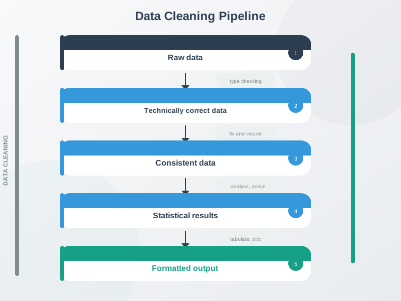
- Data Quality and Preprocessing for the wider validate-clean-transform pipeline.
- Data Validation and Outlier Detection for the checks that should run before repair.
- Data Quality Normalisation Lab for scaling clean and flagged features.
36.9 Next
Return to Imputation & Noise Filtering after the repair contract is clear, then continue to Data Quality Normalisation Lab to scale clean values without hiding repair flags.