44 Radio Gateway Aggregation
44.1 Start With the Story
Picture an IoT team using the ideas in Radio Gateway Aggregation during a live operations review. A device has produced messy evidence, an analytic step is about to change an alert or control decision, and someone has to explain why the result should be trusted.
Read this page as that path from sensor evidence to accountable action. Start with what the system observes, keep the model or data treatment visible, and finish with the check that would convince an operator, maintainer, or auditor to act.

Phoebe’s Why
Sampling is a strobe light, not a movie camera. Point a strobe at a spinning wheel and, if the flashes land at just the wrong rate, the wheel looks like it is turning slowly backward – the true fast motion has folded down into a false slow one. That is aliasing, and the only defence is the Nyquist rule: the sample rate must be at least twice the fastest rate of change you need to trust, \(f_s \geq 2f_{\max}\). A freezer sampled every 10 seconds is watching a slow compressor cycle just fine, but a fast transient such as a door left open briefly does not politely wait for the strobe – it either gets caught by luck or folds into what looks like ordinary slow drift. The ADC adds a second, smaller kind of noise on top: no matter how fast you sample, each reading is rounded to the nearest of \(2^N\) steps, and that rounding behaves like a small, fixed amount of extra noise riding on every value.
The Derivation
Nyquist criterion:
\[f_s \geq 2f_{\max}\]
Aliased frequency for an under-sampled component \(f_{\mathrm{true}}\), with \(k\) the nearest integer to \(f_{\mathrm{true}}/f_s\):
\[f_{\mathrm{alias}} = \left| f_{\mathrm{true}} - k f_s \right|\]
Quantization step and noise power for an \(N\)-bit ADC with reference \(V_{\mathrm{ref}}\):
\[q = \frac{V_{\mathrm{ref}}}{2^N}, \qquad P_{\mathrm{noise}} = \frac{q^2}{12}\]
\[\mathrm{SNR}_{\mathrm{dB}} = 6.02N + 1.76\]
Worked Numbers: The Door-Open Transient
- Baseline sample rate: \(f_s = 1/10\text{ s} = 0.1\) Hz \(\to\) Nyquist limit \(f_{\max} = 0.05\) Hz (a 20 s period)
- A brief door-open event (catalog-typical \(\approx 3\) s duration): \(f_{\mathrm{true}} \approx 1/3 = 0.333\) Hz, well above the 0.05 Hz limit
- Aliased appearance: \(k = \mathrm{round}(0.333/0.1) = 3 \to f_{\mathrm{alias}} = |0.333 - 0.3| = 0.033\) Hz, a $$30 s wobble indistinguishable from ordinary compressor drift – the transient hides in plain sight
- Quantization (12-bit ADC, 3.3 V reference, catalog-typical): \(q = 3.3/4096 = 0.806\) mV; \(\mathrm{SNR} = 6.02(12)+1.76 = 74.0\) dB
- Battery tie: fixing the alias by simply sampling fast enough everywhere needs \(f_s \geq 0.667\) Hz, i.e. a full duty cycle every 1.5 s – but even the chapter’s optimized burst (5 s active + 2 s TX = 7 s) cannot physically fit inside a 1.5 s window. That mismatch is exactly why the fix is adaptive triggering (sample cheaply and often enough to satisfy Nyquist, transmit only the rare 120 mA burst on a real event) rather than raising the whole hourly duty cycle, which is what keeps the chapter’s own 0.112 mA / 2.56-year result achievable at all
44.2 Learning Objectives
After this page, you should be able to:
- Explain why radio transmission usually dominates battery-powered edge acquisition.
- Design adaptive sampling, batching, and in-network aggregation policies that reduce uplink traffic.
- Preserve min, max, count, event flags, sequence metadata, and queue-health fields so summaries remain interpretable.
- Evaluate the latency, detail loss, and aliasing risks introduced by low-power gateway policies.
44.3 Why This Follows Edge Power and Gateways
Edge Power and Gateways teaches battery-life arithmetic, duty cycling, gateway protocol translation, store-and-forward buffering, and deployment examples. This page narrows in on the deeper contract behind those power savings: which data can be delayed, summarized, or dropped, and which metadata must travel with every gateway summary.
Use it when a site gateway or battery node must save energy without hiding a short event, creating unexplained gaps, or sending a summary the cloud cannot audit.
44.4 Radio Dominates Battery Drain
On a battery-powered sensor node, the intuition that “computing costs energy” is misleading. The real energy hog is the radio: transmitting data can cost as much energy as executing thousands of instructions. This single fact reshapes the whole acquisition strategy – the goal is to transmit less, even if that means computing more.
Consider the hourly example earlier in the chapter. A node that spends 30 seconds active at 25 mA, 10 seconds transmitting at 120 mA, and the rest asleep averages about 0.55 mA. If firmware trims that to 5 active seconds and 2 transmit seconds per hour, the average falls to about 0.112 mA. On the same 2500 mAh battery, lifetime moves from roughly 189 days to more than 2.5 years. The sensor did not become magical; it simply stopped waking and talking so often.
Three techniques follow directly: sample adaptively so you capture fewer, more useful samples; aggregate readings in the network before the uplink; and duty-cycle the radio so it is off almost all the time. A gateway reinforces the same pattern at site scale. It accepts short-range traffic from BLE, Zigbee, Modbus, or LoRa devices, performs local validation and buffering, then sends compact cloud messages instead of forcing every endpoint to hold an expensive upstream session.
Intuition: talking is expensive, thinking is cheap. A good sensor node thinks a lot – filtering, summarising, deciding – so that when it finally talks, it says something short and worth the energy.
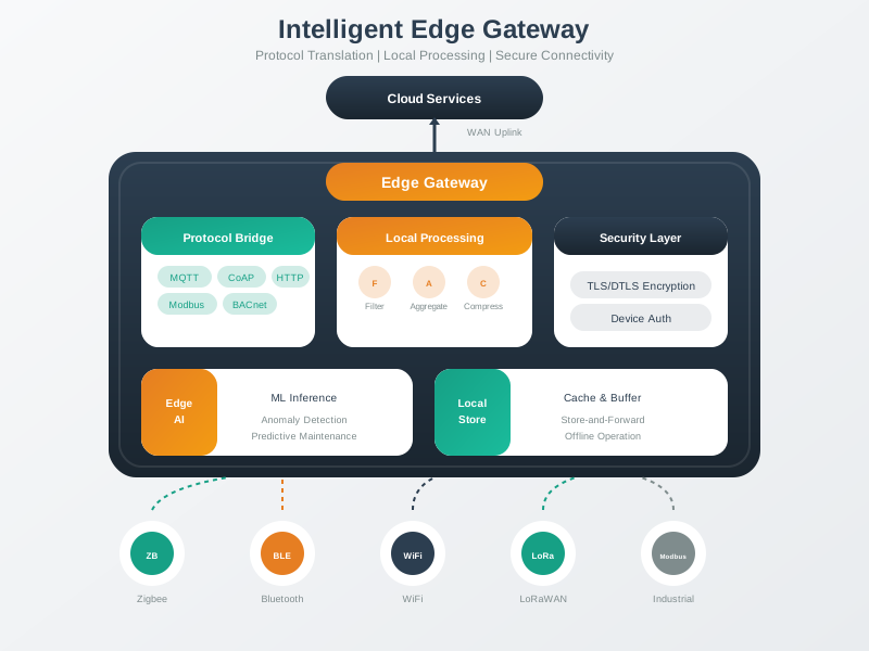
The power lesson is therefore architectural, not only electrical. The device firmware decides when to wake. The local network decides which radio path is cheap enough for the payload. The gateway decides what must cross the costly backhaul. When those three choices agree, the system preserves data quality while reducing the number, duration, and size of transmissions.
44.4.1 Overview Knowledge Check
44.5 Adaptive Sampling and Aggregation
Adaptive/event-driven sampling: sample fast when the signal changes,
   slow when stable; or send only on a significant change/threshold
In-network aggregation: the gateway combines many readings into
   summaries (mean, min, max, count) before the uplink
Duty cycling: keep radio + sensors off; wake -> sample -> batch -> send -> sleep
A practical design starts by writing the radio schedule before the analytics pipeline. For each measurement family, decide the minimum rate needed to avoid missing the phenomenon, the event trigger that justifies an immediate send, and the heartbeat interval that proves the node is still alive. A freezer temperature sensor might sample every 10 seconds locally, but send only when temperature moves more than 0.5 C, when a door-open event occurs, or when the hourly heartbeat is due. The cloud still receives enough information to reconstruct equipment state, while the radio avoids hundreds of routine packets.
The gateway then becomes the place where repeated local readings are turned into evidence. It can keep a rolling window per device, attach gateway receive time, reject malformed values, and emit a compact record such as mean, min, max, count, first time, last time, and event flags. This is not blind compression. It is a contract: the summary fields must preserve the decisions the system will make later. For maintenance dashboards, min/max and count often matter as much as the mean; for alarms, the event flag may matter more than the average.
Worked example: cutting an uplink by 20x
A temperature node sampling every 3 s = 1,200 readings/hour.

  Naive: transmit all 1,200 readings each hour.

Adaptive + aggregate at the gateway:
  - values are stable, so send only on a >0.5 C change,
    plus one heartbeat + hourly (mean, min, max, count)
  - typical hour: ~60 transmitted items instead of 1,200
  -> ~20x less radio traffic, and thus far less energy,
     while preserving the trend and the extremes.
If each raw reading is a compact 20-byte payload, the naive hour is about 24 KB before radio overhead and acknowledgements. A summary message with mean, min, max, count, timestamps, and a health flag might be under 80 bytes. Even if the summary is sent several times for reliability, the gateway has removed most uplink traffic while keeping the values needed to detect drift, excursions, and sensor silence.
Notice what is preserved: the summary keeps the mean and the min/max, so a peak is not lost even though most individual readings are never sent. Choosing which aggregates to keep is how you save energy without discarding what matters.
Implementation discipline matters. Put a maximum hold time on every batch so stale data does not wait forever for a full packet. Size the local queue for the longest expected outage plus a margin. Include sequence numbers or monotonic counters so the cloud can spot gaps after reconnect. Finally, measure current with the firmware running, because a board that looks asleep in software can still leak current through sensors, regulator quiescent draw, pull-ups, or a radio module left in idle.
44.5.1 Practitioner Knowledge Check
44.6 Energy-Saving Tradeoffs
Energy reduction is never free. It works because the system chooses which information can be delayed, summarized, or ignored. A radio wake-up has fixed overhead: the oscillator starts, the transceiver locks, the MAC may listen or join, the packet is sent, and acknowledgements or retries may follow. Batching ten readings into one wake-up can save much of that fixed cost. The price is that the first reading in the batch is older by the time the cloud sees it.
Aggregation has a different cost. A mean is compact and useful for trends, but it is lossy. If a motor bearing temperature is 40 C for 59 minutes and 95 C for one minute, the hourly mean may look harmless while the peak was the maintenance signal. That is why gateway summaries should be designed from the decision backward: include min/max for excursions, count for completeness, standard deviation for variability, and flags for threshold crossings or sensor-health events.
Adaptive sampling also needs a guardrail. A node that samples slowly during stable periods can miss a short transient if the signal changes faster than the reduced sampling rate can observe. Keep a minimum sample floor, add interrupt-style triggers where hardware supports them, and treat every sampling policy as part of the data-quality contract. The gateway can reduce data, but it should also report what it reduced and which assumptions were active.
Buffer metadata closes the loop. Each summary should carry the number of raw readings represented, the time range covered, and whether any local queue overflow, retry limit, or sensor error occurred. Without those fields, the cloud cannot distinguish “stable temperature” from “gateway dropped half the batch.” Energy savings are only useful when the downstream interpretation remains honest.
Batching costs latency
Sending many readings in one radio wake-up amortises the fixed cost of powering the radio on, but holds data back until the batch is sent. More batching means more energy saved and more delay – a direct trade-off.
Aggregation hides detail
A mean conceals the peak and the shape. Preserve what matters by also sending min, max, count, or event flags – otherwise a rare but important spike vanishes into the average.
Adaptive sampling can alias
Slowing the sample rate during a fast transient can miss or alias it (the Nyquist rule still applies). Adapt on the signal’s real dynamics and keep a minimum floor rate so fast events are not lost.
The gateway is a filter
The organising idea is data reduction close to the source: only meaningful, compact data should cross the expensive link. The gateway’s job is to decide what is worth the energy to send.
So low-power acquisition is a series of deliberate trades: batch to amortise radio wake-ups (accepting latency), aggregate to cut volume (while keeping extremes), and sample adaptively (without under-sampling transients). A useful engineering review asks four questions before approving the policy: what is the maximum delay introduced, which extremes are preserved, what event can wake the node early, and how will the cloud know a summary was incomplete? Each trade spends a little timeliness or detail to buy a lot of battery life; the right balance is set by what the application actually needs to know.
44.6.1 Under-the-Hood Knowledge Check
44.7 Release Checklist
Before shipping a low-power gateway policy, verify these records:
- Every batch has a maximum hold time, source time range, raw sample count, and sequence or monotonic counter.
- Gateway summaries preserve the decision-critical fields: min, max, count, event flags, threshold crossings, and quality markers where needed.
- Adaptive sampling has a minimum sample floor and an explicit event trigger for fast transients.
- Store-and-forward queues are sized for the longest expected outage plus margin, and queue overflow is surfaced to the cloud.
- Field current has been measured with the real firmware, sensors, regulators, and radio module states active.
44.8 See Also
- Edge Power and Gateways for battery-life arithmetic, gateway functions, and deployment examples.
- Edge Acquisition Sampling and Compression for sampling and data-reduction strategies.
- Time-Series Compression and Audit Boundaries for lossless compression and evidence grades.
- Edge Acquisition Architecture for device categories and connectivity paths.
44.9 Next
Return to Edge Power and Gateways, then continue to Edge Compute Patterns to place gateway aggregation inside a full edge design.