34 Signal Preprocessing Contracts
34.1 Start With the Story
Picture an IoT team using the ideas in Signal Preprocessing Contracts during a live operations review. A device has produced messy evidence, an analytic step is about to change an alert or control decision, and someone has to explain why the result should be trusted.
Read this page as that path from sensor evidence to accountable action. Start with what the system observes, keep the model or data treatment visible, and finish with the check that would convince an operator, maintainer, or auditor to act.
34.2 Learning Objectives
After this page, you should be able to:
- Explain why preprocessing order changes the statistical meaning of a sensor stream.
- Choose alignment, resampling, smoothing, and detrending steps based on the physical signal you must preserve.
- Identify when causal filters, centered filters, interpolation, or downsampling can mislead real-time IoT decisions.
- Record preprocessing parameters and quality flags so dashboards, models, and incident reviews can reproduce the cleaned stream.
34.3 Why Contracts Follow Workflow
Data Preprocessing Workflow teaches the full validate-clean-transform path, the cost of poor data quality, and the basic pipeline used before IoT analytics or machine learning. This page narrows in on the deeper contract behind that workflow: the order of transformations, the signal features each step can damage, and the records needed to make preprocessing auditable.
Use it when a cleaned stream feeds alarms, feature extraction, dashboards, or models where event timing and signal shape matter. A polished line is not necessarily better evidence; the workflow must preserve the events the system is supposed to detect.
34.4 Raw Data Needs Preprocessing
Between validated raw readings and a model that can learn from them sits preprocessing: aligning sensors that sample at different rates, filling or marking gaps, smoothing noise, and removing trends. Skip it and even a good model struggles, because it is fed misaligned, noisy, drifting inputs that obscure the pattern you want it to find.
Preprocessing is a workflow, not a single step, and the order of operations matters. Smoothing before removing an outlier smears that outlier into its neighbours; resampling before aligning timestamps mixes readings that never co-occurred. Getting the sequence right is as important as choosing the techniques.
Intuition: preprocessing is preparing ingredients before cooking. You wash and chop in a sensible order — and if you blend before removing the stone, the whole dish is ruined no matter how good the recipe.
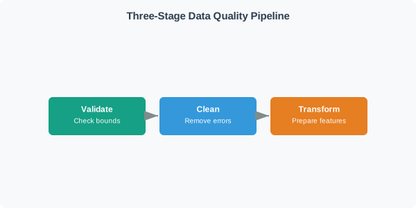
For example, a cold-room monitor might collect temperature every 10 seconds, door state every event, and compressor current once a minute. Preprocessing first brings those readings onto a common timeline, then rejects impossible values such as 900 degrees C, marks missing intervals, and smooths electrical noise without hiding a real door-open warming event. The cleaned result is still not a model input until it is transformed into features such as last five-minute mean, rate of warming, door-open count, and compressor duty cycle.
The important distinction is that preprocessing preserves evidence while making the signal usable. A removed point should leave a quality flag; an imputed value should be distinguishable from a measured value; a resampled series should record the original sampling interval. Those records let later troubleshooting answer whether an alarm came from the physical process or from the cleaning choice.
In practice, the safe workflow is boring: keep the validated raw stream, run deterministic steps in a documented order, store parameters with the model or dashboard, and review edge cases before deployment. That discipline gives downstream analytics a stable contract instead of a moving target.
Overview Knowledge Check
34.5 Align, Smooth, Resample
A practical preprocessing run starts by writing down the target analysis grain. If the model makes one prediction per minute, a 100 Hz vibration stream, a 1 Hz temperature stream, and event-driven door contacts all need rules that convert them to that one-minute grain. The conversion might be mean vibration energy, maximum temperature, door-open seconds, and the count of validation failures. Without that target grain, teams often resample blindly and create features that cannot be compared.
Choose filters from the physical event you must preserve. A moving average is acceptable for a slow room-temperature trend because a few seconds of lag may be harmless. It is a poor choice for a pressure spike, impact, or vibration peak where the height and onset time are the evidence. For those cases, a median filter may remove one-sample spikes, or a Savitzky-Golay filter may reduce noise while preserving peak shape. The filter is part of the measurement design, not cosmetic cleanup.
Align/resample: put sensors on a common time grid (interpolate up,
                aggregate down) so readings are comparable
Smooth noise:   moving average (simple, but lags and blurs edges)
                Savitzky-Golay (fits a small polynomial per window ->
                smooths while preserving peaks and slopes)
Detrend:        remove slow drift so the pattern of interest stands out
Worked example: moving average vs Savitzky-Golay
A signal with a sharp genuine peak plus noise:

  Moving average (window 11): flattens the noise AND the peak,
     and shifts features slightly (it lags).
  Savitzky-Golay (window 11, order 3): fits a cubic in each
     window, so it removes noise while keeping the peak's height
     and the slopes on either side.

Choose the smoother by what you must preserve: moving average
for a stable level, Savitzky-Golay when peak shape/derivatives matter.
A sensible default order is: validate, remove or flag outliers, align/resample onto a common grid, then smooth, then detrend. Each step assumes the previous one has already run.
Before handing features to a model, run a small audit table for each feature: raw source, validation rule, imputation rule, resampling rule, filter window, and whether the feature can be computed online. That table catches common production mistakes, such as using future samples in a centred smoothing window for a real-time alarm, or recomputing normalization statistics from each incoming batch instead of using the training parameters.
For edge devices, start with integer-friendly checks and bounded memory. A ring buffer of 30 samples is enough for many rolling means, medians, and rate-of-change checks. If a transform needs a long window, a floating-point library, or a cloud lookup, treat that as an explicit architecture decision and measure the latency and power cost.
Practitioner Knowledge Check
34.6 How Preprocessing Misleads
Preprocessing changes the statistical meaning of the data. A moving average reduces variance, interpolation creates synthetic samples, detrending removes low-frequency content, and downsampling discards information above the new sampling limit. These changes may be exactly what the analysis needs, but they must be visible because the model now sees a constructed signal rather than the raw sensor stream.
The timing model is just as important as the math. Offline analysis can use centred windows or zero-phase filters because it can look forward and backward around an event. A live edge alarm cannot use future samples without delaying the alert or leaking future information into the decision. If a filter needs five future samples to look clean in a notebook, it is not the same filter that can run in production at the event boundary.
Aliasing is the other hidden trap. If a 100 Hz vibration component is downsampled to 20 Hz without a low-pass filter, high-frequency energy folds into lower frequencies and can look like a real slow oscillation. The pipeline may appear smoother and cheaper, while the feature has become false evidence. Downsample only after filtering out content the new sample rate cannot represent.
Finally, preprocessing choices must be versioned. Changing an imputation window, a smoothing alpha, or a normalization range can shift model inputs enough to invalidate comparisons with previous metrics. Store the transform version alongside the output so a dashboard change, model drift, or incident review can be traced to the exact preprocessing rules used. That record also lets teams rerun old raw data through the new pipeline and measure whether the change improved the signal or only moved the baseline.
Smoothing adds lag
Every causal smoother delays the signal, because it averages in past samples. For real-time alarms that lag can be the difference between catching an event and missing its onset; account for it or use a zero-phase filter offline.
Resampling is not free
Upsampling invents points by interpolation (which can imply detail that was never measured); downsampling must respect the sampling limit to avoid aliasing. Neither creates information that was not sampled.
Over-smoothing hides signal
Too wide a window erases the very features you are trying to detect. The window should be matched to the timescale of the phenomenon, not set to “as smooth as possible”.
Keep a raw copy
Preprocessing is lossy and choices are revisited. Retain the validated raw data so you can reprocess with different parameters instead of being stuck with one irreversible pipeline.
So preprocessing is a careful sequence of lossy transformations, each of which can help or mislead: align first so comparisons are valid, smooth with a filter and window matched to what you must preserve, detrend to expose the pattern, and keep the raw data so the choices remain reversible. The goal is to clarify the signal, never to manufacture one.

Phoebe’s Why
A sampled stream is not the signal – it is the signal’s value at a fixed grid of instants. If the signal wiggles faster than that grid can track, two different wiggles can leave the exact same trail of samples, and nothing in the data says which one really happened. That confusion is aliasing: a fast oscillation impersonates a slow one because the sampler only ever sees the grid points, never the path in between. The Nyquist criterion removes the ambiguity – sample at least twice per cycle of the fastest content present, and no slower wiggle could have left the same trail. Quantization is a second, independent kind of loss: even a perfectly timed sample still gets rounded to the nearest of \(2^N\) codes, so a small, fixed error rides along with every reading no matter how carefully the timing was chosen.
The Derivation
For a signal whose fastest component is \(f_{max}\), faithful sampling requires
\[f_s \geq 2f_{max}\]
Sampling at \(f_s\) replicates the signal’s spectrum at every multiple of \(f_s\). If \(f_s < 2f_{max}\), the replica centred on \(f_s\) overlaps the original, and a component at \(f\) reappears at
\[f_{alias} = \left| f - n f_s \right|, \quad n = \mathrm{round}(f/f_s)\]
indistinguishable from a real low-frequency signal.
Quantization to \(N\) bits over range \(V_{ref}\) leaves a rounding error \(e\) uniform on \([-q/2,+q/2]\), with step \(q = V_{ref}/2^N\):
\[\overline{e^2} = \frac{1}{q}\int_{-q/2}^{+q/2} x^2\,dx = \frac{q^2}{12}\]
\[\mathrm{SNR} = 10\log_{10}\!\left(\frac{V_{ref}^2/8}{q^2/12}\right) \approx 6.02N + 1.76\text{ dB}\]
Worked Numbers: This Chapter’s Streams
- The chapter’s own case: a 100 Hz vibration component downsampled to 20 Hz needs \(f_s \geq 2\times100 = 200\) Hz to stay faithful; 20 Hz is only \(20/200 = 0.1\times\) that requirement – a 10x shortfall.
- Alias location: \(n = \mathrm{round}(100/20) = 5\), so \(f_{alias} = |100 - 5\times20| = 0\) Hz. Because 100 Hz is an exact multiple of the 20 Hz grid, this component does not fold to a beat frequency – it folds straight to a DC offset, which can look like slow sensor drift rather than a vibration event at all.
- By contrast, the chapter’s 1 Hz temperature stream is comfortably sampled: as long as the true thermal signal changes slower than \(f_s/2 = 0.5\) Hz, Nyquist holds with room to spare, which is why smoothing lag (not aliasing) is the main risk called out for that channel.
- Quantization: the chapter does not name a converter, so take a standard 10-bit ADC referenced to 3.3 V (a typical low-cost data-logger front end). \(q = 3.3/2^{10} = 3.22\) mV; RMS quantization noise \(q/\sqrt{12} = 0.930\) mV; ideal \(\mathrm{SNR} = 6.02(10)+1.76 = 62.0\) dB.
A downsample step is a second, silent sampler riding on top of the first. It needs its own anti-alias low-pass filter, sized to the new \(f_s/2\), applied before the decimation – the same Nyquist guarantee the original ADC needed, reapplied at every rate change in the pipeline.
Under-the-Hood Knowledge Check
34.7 Release Checklist
Before shipping a preprocessing workflow, verify these records:
- The raw stream, validated stream, cleaned stream, and feature stream are separately retained or reproducibly derivable.
- Every transform names its order, parameters, window length, sample rate, and online/offline timing assumption.
- Imputed, filtered, rejected, and resampled values keep quality flags and source timestamps.
- Smoothing and resampling have been checked against the event shape, timing, and frequency content the application must preserve.
- Dashboard, model, and incident-review artifacts record the preprocessing version used to create their inputs.
34.8 See Also
- Data Preprocessing Workflow for the full validate-clean-transform overview.
- Missing Value Imputation and Noise Filtering for gap filling and repair strategies.
- Feature Scaling and Leakage Controls for transform-parameter provenance.
- Modeling Feature Engineering for downstream model inputs.
34.9 Next
Return to Data Preprocessing Workflow, then continue to Missing Value Imputation and Noise Filtering for the cleaning stage details.