Chapters

52 Big Data Fundamentals

analytics-ml
big
data

52.1 Begin With One Day of Device Records

Telemetry means records sent from a system so its state can be watched. Picture ten thousand meters that each send a small reading once a minute. The first choice is not a brand of data tool. It is the work the records must support and the time, quality, and keep rules that work needs.

Count devices, bytes per record, and records per hour. Add late, repeated, and missing events. Mark which time comes from the device and which comes from arrival. Then follow one record through intake, check, store, query, and removal. Test a burst, a slow stage, a bad clock, and a lost link. Record what waits, what is dropped, and how the team knows.

Keeping more can help later study, but it raises cost, privacy, and search load. Fast intake can protect fresh work, but it may pass poor data unless checks keep up. A large count alone does not make a sound design. Use the Practitioner layer to size the stages and choose controls. Use the Under the Hood layer to inspect event time, state, replay, backpressure, and recovery. Those routes turn the simple daily count into an honest service contract.

52.2 Start With the Story

Picture an IoT team using the ideas in Big Data Fundamentals during a live operations review. A device has produced messy evidence, an analytic step is about to change an alert or control decision, and someone has to explain why the result should be trusted.

Read this page as that path from sensor evidence to accountable action. Start with what the system observes, keep the model or data treatment visible, and finish with the check that would convince an operator, maintainer, or auditor to act.

52.3 Big Data as Engineering Contract

Big data in IoT is not just a synonym for a large database. It describes a workload whose size, arrival rate, format mix, quality risk, and decision value shape the architecture. A temperature history table, a vibration stream, a fleet of camera summaries, and a connected-vehicle telemetry feed can all be "big" for different reasons.

Where the Flood Comes From

Big data did not start big. Figure 52.1 shows the world it replaced: three information services, each with its own dedicated delivery network and its own physical medium.

Three lanes: office computers exchange email over a computer network on copper or fibre; desk telephones carry a voice call over the telephone network on twisted pair; a TV studio broadcasts one way to home televisions over aerial or satellite. A trade-off card notes that isolation keeps each service simple but capacity cannot be shared and IoT telemetry would need a fourth build.
Figure 52.1: Before convergence: computer, telephone, and broadcast services each ran on a dedicated network.

The lane worth pausing on in Figure 52.1 is the bottom one: the Broadcast network transmits one way only, which is why its receiver card simply shows the programme while the computer and telephone lanes exchange traffic in both directions. The THE TRADE-OFF card underneath states the economics that killed this model — every new service, IoT telemetry included, would have demanded yet another dedicated build.

Convergence answers that trade-off. In Figure 52.2 the same endpoints — now joined by IoT sensors — share a single IP network, and the centre of the diagram shows what that sharing physically means.

Four sources — computer, IP telephone, smart TV, IoT sensors — connect to one converged IP network where packets from every service interleave on the same pipe before reaching the email server, call peer, streaming service, and IoT platform. A trade-off card warns that services share capacity and fate, making prioritisation a design duty.
Figure 52.2: After convergence: one IP network carries email, voice, video, and IoT telemetry on shared capacity.

Look inside the Converged IP network block of Figure 52.2: the interleaved packet strip is the whole story, because congestion in the pipe touches all four services at once. The trade-off flipped rather than vanished — separate networks wasted capacity, the converged network shares fate, and the IoT platform at the lower right now competes with video for the same pipe. Prioritisation therefore appears in the figure as a design duty, not an optional extra.

Once every service travels as digital traffic, the stored record of the world turns digital too. Figure 52.3 puts measured numbers on how quickly that happened.

Five 100-percent stacked columns show the digital share of global storage rising from 1 percent in 1986 and 3 percent in 1993 to 25 percent in 2000, a 50-50 crossover in 2002 labelled the beginning of the digital age, and 94 percent in 2007, when 280 exabytes were digital and 19 exabytes analog. Data from Hilbert and Lopez, Science 2011.
Figure 52.3: Global storage capacity flipped from 99% analog in 1986 to 94% digital by 2007.

Hold the two end columns of Figure 52.3 against each other: 1986 stored 2.6 EB in total, 99 % of it analog, while 2007 stored digital 280 EB against analog 19 EB — roughly a hundredfold expansion in which the digital share crossed 50 % only in 2002. Sensor fleets extend exactly this curve, which is why the rest of this chapter turns the vocabulary of scale into an engineering contract instead of a slogan.

The common shorthand is the 5 Vs: volume, velocity, variety, veracity, and value. They become useful when each V turns into a design requirement. Volume asks how many bytes and records must be retained. Velocity asks how quickly events arrive and how soon they must affect a decision. Variety asks how many schemas, units, media types, and device models must be combined. Veracity asks how the system handles missing, duplicated, noisy, late, or drifting data. Value asks what decision justifies the cost.

A useful IoT big-data statement is specific: "10,000 sensors publish one 80-byte reading per second; operations needs one-minute alerts, 30 days of raw replay, and one year of hourly aggregates." That statement is easier to design from than "we have lots of data."

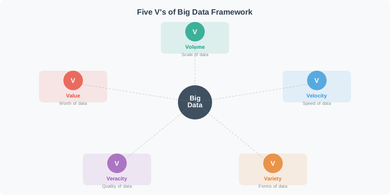
Use the five-V diagram in Figure 52.4 to turn the familiar vocabulary into a review of the system's actual pressures.

Five Vs of Big Data framework: Big Data sits in the center, connected to Volume as scale of data, Velocity as speed of data, Variety as forms of data, Veracity as quality of data, and Value as worth of data.
Figure 52.4: The Five Vs are useful when each one becomes a design pressure: storage scale, arrival speed, format diversity, evidence quality, and the decision value that justifies the pipeline.

Read Figure 52.4 around the centre rather than as a ranked list. Volume asks how much must be stored or scanned; velocity asks how quickly it arrives and must influence a decision; variety exposes schema and semantic differences; veracity tests whether observations can be trusted; value names the decision worth supporting. The centre matters because the pressures interact. This advances the running narrative from a data-size label to an engineering contract with measurable ingest, quality, retention, and outcome requirements.

52.4 When the Source Uses Seven Vs

The NPTEL source uses a seven-V vocabulary: volume, velocity, variety, variability, veracity, visualization, and value. Its two additional labels make useful review questions without replacing this chapter’s five-part engineering contract. Variability asks whether meaning changes with context, as it can for language, hashtags, geospatial data, multimedia, or sensor events. Visualization asks whether a pictorial or graphical presentation helps a decision-maker see an analytic result or pattern. In this chapter’s workflow, record variability under the schema-and-context work prompted by variety, and treat visualization as a delivery check between analysis and decision. The important evidence is the requirement each label exposes, not whether a team says “five” or “seven.”

Volume

How many records and bytes arrive, and how long raw, cleaned, and aggregated data must be retained.

Velocity

How quickly events arrive, queue, and need to be transformed into alerts, dashboards, or control actions.

Variety

The mix of MQTT payloads, JSON logs, binary samples, Parquet batches, images, device metadata, and units.

Veracity

The trust controls for duplicates, gaps, calibration drift, schema drift, outliers, and late-arriving events.

Value

The operational decision: detect faults, reduce energy use, schedule maintenance, document compliance, or improve a product.

V
Question
IoT Example
Architecture Consequence
Volume
How much raw and derived data must be stored?
Industrial sensors emit a steady stream plus bursty diagnostics.
Partition by device, site, and time; move cold data to object storage.
Velocity
How long can events wait before the decision is stale?
Motor vibration anomalies may need seconds, while monthly reports can wait.
Use stream processing, backpressure, and bounded-latency alerts.
Variety
How many formats and schemas must be reconciled?
MQTT telemetry, gateway logs, maintenance tickets, and image labels.
Use schema registry, explicit units, and typed raw-to-curated zones.
Veracity
Can the system tell trustworthy readings from bad evidence?
Sensor drift, retransmitted messages, clock skew, and missing windows.
Validate at ingestion, keep quality flags, and design idempotent writes.
Value
Which decision pays for collection and processing?
Predictive maintenance saves downtime only when alerts are timely and reliable.
Measure data products by decision accuracy, latency, and cost, not just storage size.

Overview Knowledge Check

52.5 Size Pipeline Before Tools

Start with the event contract: timestamp, device id, schema version, units, quality flags, and payload size. Then size the pipeline from the outside in. MQTT, HTTP, or gateway protocols deliver events to an ingestion service; Apache Kafka or a cloud equivalent buffers and partitions streams; Spark Structured Streaming, Apache Flink, or a managed stream processor computes windows; curated data lands in a time-series database, lakehouse table, or object store such as Parquet files in cloud storage.

The tool names matter only after the workload is sized. A small campus deployment may work with a time-series database and nightly Parquet export. A regional fleet may need Kafka partitions, schema registry, stream processors, and a raw/curated data lake. The design mistake is choosing a large stack because the phrase "big data" sounds impressive, or choosing a single server when the rate and retention math already shows a distributed workload.

Worked example: rate, volume, and retention
fleet size: 10,000 sensors
publish rate: 1 reading per second per sensor
payload after protocol parsing: 80 bytes per reading

events per second:
10,000 sensors * 1 reading/s = 10,000 events/s

ingest bytes per second:
10,000 events/s * 80 bytes = 800,000 bytes/s
800,000 bytes/s = 0.8 MB/s using decimal units

daily raw volume:
0.8 MB/s * 86,400 s/day = 69,120 MB/day = 69.12 GB/day

30-day raw retention:
69.12 GB/day * 30 = 2,073.6 GB, or about 2.07 TB

hourly aggregate retention:
10,000 sensors * 24 hourly records/day * 120 bytes = 28,800,000 bytes/day
28,800,000 bytes/day = 28.8 MB/day

design implication:
Keep raw records for replay and debugging while they are operationally useful.
Keep compact aggregates much longer for dashboards, reports, and trend models.

Partitioning is part of the data model. Kafka partitions, Parquet folder layout, and database shard keys should spread load across time and devices. A poor key can create a hot partition even when the total cluster size looks adequate.

Layer
Typical Technology
Design Choice
Failure to Avoid
Device ingress
MQTT broker, HTTP endpoint, gateway agent, or cloud IoT hub.
Set device identity, timestamp source, payload schema, and retry behavior.
Accepting messages without units, schema version, or quality context.
Stream buffer
Apache Kafka, Redpanda, Pulsar, or managed cloud streams.
Partition by a key that balances load while preserving needed ordering.
Putting all traffic for a busy site or device type into one partition.
Processing
Spark Structured Streaming, Apache Flink, Beam, or cloud stream jobs.
Choose tumbling, sliding, or session windows with watermarks for late data.
Using processing time when event time is required for correct windows.
Storage
Time-series DB, lakehouse tables, Parquet in object storage, Delta Lake, or Iceberg.
Separate raw, cleaned, aggregated, and serving-ready zones.
Overwriting evidence needed for replay, audit, or model debugging.

Practitioner Knowledge Check

52.6 Time, State, and Backpressure

At scale, IoT big-data errors often come from timing and state rather than from the storage engine itself. Devices report event time, gateways add arrival time, brokers preserve ordering only within a partition, and stream processors must decide when a window is complete. Late events, clock skew, duplicate retries, and out-of-order batches can make a dashboard or alert incorrect unless the pipeline treats time as part of the data contract.

Watermarks tell a stream processor how long to wait for late data before closing a window. Idempotent writes keep retries from double-counting the same reading. Schema evolution rules prevent a new firmware version from silently breaking downstream jobs. Backpressure tells upstream components that the sink is slower than the source so the system can buffer, scale, sample, or shed noncritical work instead of failing unpredictably.

Worked example: velocity and backpressure
gateway ingest rate: 12,000 events/s
current sink write rate: 9,000 events/s

backlog growth:
12,000 - 9,000 = 3,000 events/s

after 10 minutes:
3,000 events/s * 600 s = 1,800,000 queued events

if each event averages 120 bytes after enrichment:
1,800,000 * 120 bytes = 216,000,000 bytes, or 216 MB

design implication:
A short sink slowdown can create a large queue. The pipeline needs lag alarms,
autoscaling rules, replay capacity, and a policy for dropping or downsampling
noncritical streams before critical alerts are affected.

Event Time

The timestamp when the reading was measured. Use it for physical windows, trends, and anomaly evidence.

Arrival Time

The timestamp when the platform received the event. Use it for lag monitoring and operations.

Watermark

The processor's estimate that older late events are unlikely enough to close a window.

Idempotency

A write design where replaying the same event does not create duplicate facts or double-counted totals.

Problem
Symptom
Control
Technology Tie-In
Late data
Window totals change after a dashboard or alert has already used them.
Use event-time windows, watermarks, allowed lateness, and correction records.
Flink and Spark Structured Streaming both support event-time windows and watermarks.
Duplicate retries
A device resend makes one physical reading count twice.
Use event ids, deterministic upserts, deduplication windows, and idempotent sinks.
Kafka keys, transactional writes, Delta Lake, and Iceberg can support replay-safe pipelines when configured carefully.
Schema drift
A firmware update changes a field name, unit, or enum value.
Version schemas, validate at ingress, and reject or quarantine incompatible events.
Schema Registry with Avro, Protobuf, or JSON Schema makes compatibility visible before deployment.
Hot partitions
One broker partition or storage shard lags while the cluster looks underused.
Choose partition keys that spread writes and preserve only the ordering that is actually needed.
Kafka partitions, object-store folder layout, and time-series database shards all need balanced keys.

Under the Hood Knowledge Check

52.7 Summary

Big data in IoT is an engineering contract about rate, size, format, quality, and decision value. The 5 Vs are useful when they become concrete numbers and controls: bytes per event, events per second, retention windows, schema versions, quality flags, event-time handling, and the operational decision the data supports. A good design sizes the workload first, then chooses tools such as MQTT, Kafka, Spark Structured Streaming, Flink, Parquet, object storage, lakehouse tables, or a time-series database to match the required latency and retention.

Key Takeaway

Do not call a workload “big data” and jump straight to a stack. Calculate event rate, daily volume, retention, aggregate size, late-data behavior, and backpressure limits. Those numbers determine whether the system needs a simple database, a stream buffer, a distributed processor, a lakehouse, or a combination of all four.

52.8 See Also

Big Data Technologies

Compare IoT big-data technologies for ingestion, brokers, storage, stream processing, batch jobs, analytics, governance, and operational fit.

Big Data Pipelines

Design big-data pipelines for IoT ingestion, buffering, transformation, enrichment, storage, stream processing, quality checks, and evidence handoff.

Big Data Operations

Operate IoT big-data systems with ingestion checks, storage lifecycle, schema control, observability, cost, reliability, governance, and retests.

Big Data Edge Processing

Explain edge processing for IoT big data through local filtering, aggregation, compression, latency control, bandwidth limits, and cloud handoff.