Picture an IoT team using the ideas in Edge Power and Gateways during a live operations review. A device has produced messy evidence, an analytic step is about to change an alert or control decision, and someone has to explain why the result should be trusted.
Read this page as that path from sensor evidence to accountable action. Start with what the system observes, keep the model or data treatment visible, and finish with the check that would convince an operator, maintainer, or auditor to act.
In 60 Seconds
Battery life is the primary constraint for most IoT edge devices. Through duty cycling – alternating between short active/transmit periods and long deep sleep periods – a device’s battery life can be extended from months to years (4-5x improvement). Gateways bridge non-IP sensors to the internet by providing protocol translation, store-and-forward buffering during outages, and security functions.
Chapter Roadmap
This chapter has two linked jobs:
First turn active, transmit, and sleep current into a battery-life ledger.
Then optimize the duty cycle and test it with the calculator.
Next move from devices to gateways: translation, buffering, security, and missing-data handling.
Finally pressure-test the ideas with vineyard, LoRaWAN, wildlife collar, and store-and-forward cases.
Checkpoints recap the main decisions. Optional calculation panels can be collapsed on a first read.
43.2 Learning Objectives
By the end of this chapter, you will be able to:
Calculate Power Budgets: Compute battery life for IoT devices based on duty cycling and transmission patterns
Design Duty Cycling Strategies: Configure active, transmit, and sleep cycles and evaluate their impact on battery longevity
Explain Gateway Functions: Describe how gateways enable non-IP devices to participate in IoT networks through protocol translation
Implement Store-and-Forward: Design and assess reliable data pipelines that survive network outages
For Beginners: Edge Data Acquisition
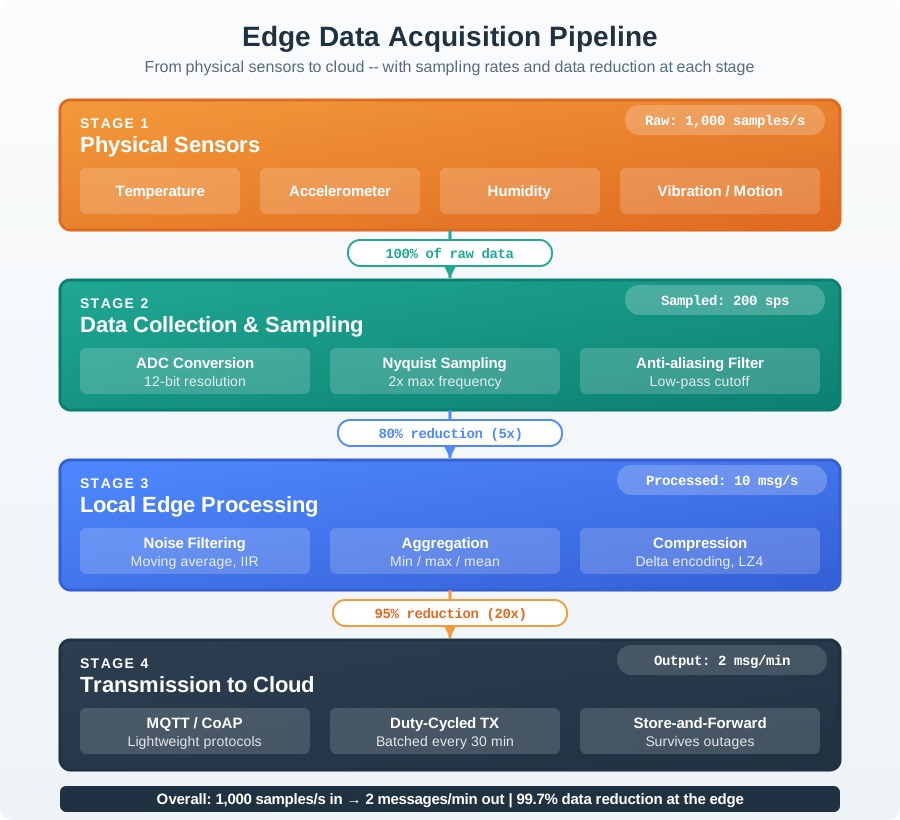
Edge data acquisition is about collecting and pre-processing sensor data right where the devices are, before sending it to the cloud. Think of a smart mailroom that sorts and summarizes incoming letters instead of forwarding every piece of junk mail to the CEO. This local filtering saves bandwidth, reduces costs, and speeds up responses.
43.3 Prerequisites
Before diving into this chapter, you should be familiar with:
Basic electrical concepts: Familiarity with current, voltage, and power calculations
43.4 Power Management and Duty Cycling
Time: ~15 min | Difficulty: Advanced | Reference: P10.C08.U04
Start with the device: every gateway promise depends on a node that wakes, measures, transmits, and sleeps again.
Key Concepts
Energy harvesting: Generating power for edge devices from ambient sources (solar, vibration, thermal gradients, RF) to enable autonomous operation in locations without permanent power infrastructure.
Duty cycling: Periodically powering down sensor hardware and radio between measurements to dramatically reduce average current consumption, extending battery life from days to years.
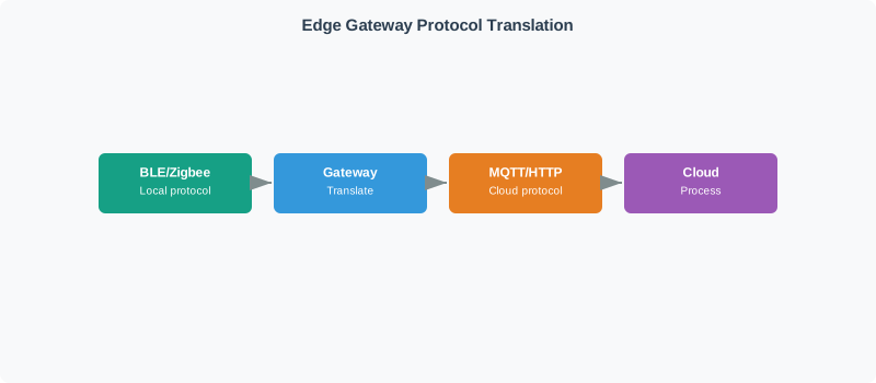
Gateway protocol translation: Converting between device-side protocols (BLE, Zigbee, Modbus) and cloud-side protocols (MQTT, HTTPS, AMQP) at the gateway, enabling heterogeneous device ecosystems to integrate with standard cloud platforms.
Store-and-forward: A gateway capability that buffers sensor data locally during connectivity outages and transmits it to the cloud when connectivity is restored, preventing data loss during network failures.
Power budget analysis: A calculation determining the average power consumption of an edge device across all operating modes (active sensing, radio transmission, sleep) to estimate battery life or harvesting requirements.
Watchdog timer: A hardware timer that resets the microcontroller if not periodically refreshed by the application, providing automatic recovery from software hangs in unattended edge deployments.
Battery life is the primary constraint for most edge IoT devices. Understanding power consumption patterns is essential for designing practical systems.
43.4.1 Power States
Most IoT microcontrollers support multiple power states:
\(t_{active}\) = time in active mode (sensing, processing)
\(t_{tx}\) = time transmitting
\(t_{sleep}\) = time in sleep mode
\(I_{active}\), \(I_{tx}\), \(I_{sleep}\) = current draw in each mode
Battery life calculation:
\[Life_{hours} = \frac{Battery_{mAh}}{I_{avg}}\]
43.4.3 Example Calculation
Scenario: ESP32 with 2500 mAh battery
Mode
Duration (per hour)
Current
Energy Contribution
Active
30 seconds
25 mA
0.208 mAh
Transmit
10 seconds
120 mA
0.333 mAh
Deep Sleep
3560 seconds
0.01 mA
0.010 mAh
Average current: (30 x 25 + 10 x 120 + 3560 x 0.01) / 3600 = 0.55 mA
Battery life: 2500 mAh / 0.55 mA = 4,545 hours = 189 days
43.4.4 Optimized Design
Reduce active to 5 seconds, transmit to 2 seconds:
Mode
Duration (per hour)
Current
Energy Contribution
Active
5 seconds
25 mA
0.035 mAh
Transmit
2 seconds
120 mA
0.067 mAh
Deep Sleep
3593 seconds
0.01 mA
0.010 mAh
Average current: (5 x 25 + 2 x 120 + 3593 x 0.01) / 3600 = 0.112 mA
Battery life: 2500 mAh / 0.112 mA = 22,321 hours = 2.5 years
Improvement factor: 4.9x (from ~6 months to 2.5+ years)
Phoebe’s Field Notes: Why Battery Life Is a Charge Ledger
Phoebe’s Why
A battery-life table is not magic bookkeeping. Current is charge flow, so every active, radio, and sleep state spends a slice of the finite charge stored in the cell. The sensor reading also has physics behind it: a transducer turns the measured condition into an electrical variable, and the node must bias that sensor, sample it, and ship the result. That is why reducing the radio burst or sensor-on time changes lifetime directly, while a high sleep current or cold derating can erase an optimistic datasheet budget.
The Derivation
Current is charge per time:
\[I = \frac{dQ}{dt}\]
For a state held for \(\Delta t\) seconds:
\[Q_{state} = I_{state}\frac{\Delta t}{3600}\]
The hourly charge ledger is:
\[Q_h = \sum I_i\frac{t_i}{3600}\]
Since one hour is the accounting interval, the average current is:
\[I_{avg} = Q_h\ \text{mA}\]
Battery lifetime follows from usable charge:
\[t_{life} = \frac{C_{usable}}{I_{avg}}\]
Energy adds voltage:
\[E_{Wh} = V\frac{C_{mAh}}{1000}\]
Under load, internal resistance lowers the terminal voltage:
\[V_{load} = V_{oc} - I R_{int}\]
The chapter does not give pack internal resistance or self-discharge, so those stay as design-check terms: \(R_{int}\) for voltage sag and \(I_{sd}\) added to the sleep ledger.
Worked Numbers: This Chapter’s Duty Cycle
Baseline ledger: active \(30\times25/3600 = 0.208\) mAh, transmit \(10\times120/3600 = 0.333\) mAh, sleep \(3560\times0.01/3600 = 0.00989\) mAh, so \(I_{avg}=0.552\) mA.
Baseline life:\(2500/0.552 = 4530\) h \(= 189\) days. The chapter’s 4,545 h comes from dividing by the rounded display value 0.55 mA.
Optimized ledger: active \(5\times25/3600 = 0.0347\) mAh, transmit \(2\times120/3600 = 0.0667\) mAh, sleep \(3593\times0.01/3600 = 0.00998\) mAh, so \(I_{avg}=0.111\) mA.
Optimized life:\(2500/0.111 = 22400\) h \(= 935\) days \(= 2.56\) years; improvement \(0.552/0.111 = 4.95\times\).
Vineyard derating check: the chapter’s 6600 mAh at 3 V stores \(6.60\times3 = 19.8\) Wh before losses. A 40% cold derating leaves \(3960\) mAh, or \(3.96\times3 = 11.9\) Wh, before voltage sag and self-discharge are subtracted.
The physical lesson is that mAh is charge, Wh is energy, and usable lifetime is the measured charge ledger after the cell’s voltage, temperature, internal resistance, and leakage have had their say.
43.4.5 Interactive Battery Life Calculator
Use this calculator to explore how duty cycling parameters affect battery life. Adjust active time, transmit time, current draw, and battery capacity to see real-time results.
Show code
viewof eapgBatteryCapacity = Inputs.range([500,20000], {value:2500,step:100,label:"Battery capacity (mAh)"})viewof eapgActiveTime = Inputs.range([1,120], {value:30,step:1,label:"Active time per hour (seconds)"})viewof eapgActiveCurrent = Inputs.range([1,250], {value:25,step:1,label:"Active current (mA)"})viewof eapgTxTime = Inputs.range([1,60], {value:10,step:1,label:"Transmit time per hour (seconds)"})viewof eapgTxCurrent = Inputs.range([50,500], {value:120,step:5,label:"Transmit current (mA)"})viewof eapgSleepCurrent = Inputs.range([0.001,1], {value:0.01,step:0.001,label:"Sleep current (mA)"})
For an ESP32 with LoRa module transmitting 50 bytes: - Deep sleep: 10 µA × 3600s = 0.01 mAh/hour - Active (sensing): 80 mA × 5s = 0.111 mAh per activation - LoRa TX (SF7, +14dBm): 120 mA × 2s = 0.067 mAh per transmission
Energy per transmission:\(E_{tx} = 120 \text{ mA} \times 2 \text{ s} = 0.067 \text{ mAh}\)
Energy per sensing:\(E_{sense} = 80 \text{ mA} \times 5 \text{ s} = 0.111 \text{ mAh}\)
Total active energy:\(0.067 + 0.111 = 0.178 \text{ mAh}\) per cycle
TX represents \(\frac{0.067 \times 12}{2.14} = 38\%\) of total energy
Batching strategy: Transmit 6 readings once per 30 min (2×/hour) instead of 12×/hour: - Active/TX energy: \(0.178 \times 2 = 0.36 \text{ mAh/hour}\) - Battery life improves by \(\frac{2.14}{0.36} = 6.0\times\)
Radio dominates because TX power (120 mA) is 12× higher than active CPU (10 mA baseline), even though TX duration is shorter.
Checkpoint: Duty-Cycle Ledger
You now know:
Baseline: 0.55 mA average gives 4,545 hours, or 189 days, from 2500 mAh.
Optimized: 5 seconds active and 2 seconds transmit drops average current to 0.112 mA.
Result: 22,321 hours, about 2.5 years, or 4.9x better than baseline.
43.5 Knowledge Check: Battery Life
43.6 Quiz 1: Battery Life Calculation
43.7 Gateway Functions for Non-IP Devices
Time: ~10 min | Difficulty: Intermediate | Reference: P10.C08.U05
Once the node can survive on battery, ask whether its data can cross protocols and outages.
Gateways serve as critical bridges between non-IP devices and the internet. Key functions include:
43.7.1 Protocol Translation
Convert sensor-specific protocols (Modbus, BACnet, Zigbee) to IP protocols
Translate between MQTT, CoAP, and HTTP as needed
Handle message format conversion (binary to JSON)
43.7.2 Data Buffering
Store data during network outages
Batch multiple sensor readings for efficient transmission
Implement store-and-forward for intermittent connectivity
43.7.3 Security Functions
Encrypt data before transmission to cloud
Authenticate devices and manage credentials
Filter and validate incoming commands
Figure 43.1: Edge Gateway Protocol Translation and Cloud Connectivity
43.7.4 Fail-Closed Gateway Admission Control
For industrial or safety-critical gateways, security should start before the protocol bridge accepts a device. A fail-closed gateway uses a default-deny policy:
Check the device identity first, such as an approved MAC address, serial number, certificate, or provisioning record.
Reject and log unknown devices before TLS or application traffic begins.
Start the TLS or mTLS handshake only for approved devices.
Apply command filtering and payload validation before forwarding data to the cloud or issuing actuator commands.
Choice
Use when
Risk if chosen poorly
Fail-closed whitelist
Critical infrastructure, industrial gateways, small controlled fleets
Stale allow-lists can block legitimate replacements until provisioning is updated.
Fail-open blacklist
Consumer or rapidly changing fleets where onboarding speed dominates
Unknown or cloned devices may connect before they are explicitly blocked.
Encryption protects data confidentiality, but it does not prove device identity by itself. A gateway that validates identity, encrypts transport, and rejects unknown devices before forwarding traffic has a smaller attack surface than a gateway that only wraps every connection in TLS.
Checkpoint: Gateway Responsibilities
You now know:
Protocol translation maps Modbus, BACnet, and Zigbee into MQTT, HTTPS, or AMQP.
Store-and-forward keeps readings during outages instead of losing the time window.
Fail-closed admission checks identity first, rejects unknown devices, then starts TLS or mTLS.
43.8 Handling Missing Data
Time: ~8 min | Difficulty: Intermediate | Reference: P10.C08.U05b
Common Pitfall: Missing Data Deletion
The mistake: Deleting rows with missing sensor values instead of using appropriate imputation or flagging strategies, losing valuable contextual information.
Symptoms:
Dataset shrinks dramatically after preprocessing (e.g., 1M rows becomes 200K)
Model accuracy drops when deployed despite good validation scores
Time gaps in data break time-series analysis (autocorrelation, windowing)
Critical events during sensor outages are completely missed
Why it happens: Beginners apply pandas dropna() liberally. In IoT, sensors fail intermittently due to battery depletion, network issues, or environmental factors. Deleting these rows removes entire time windows, including valid data from other sensors.
The fix: Use context-appropriate imputation strategies:
# For slow-changing values (temperature): forward-filldf['temp'] = df['temp'].ffill(limit=60) # Max 60 missing samples# For periodic values: interpolationdf['humidity'] = df['humidity'].interpolate(method='time')# For event-driven sensors: mark as "no event" vs "missing"df['motion_event'] = df['motion'].fillna(0) # No motion detecteddf['motion_missing'] = df['motion'].isna() # Track sensor status# For critical analysis: flag and include in modeldf['has_missing'] = df.isna().any(axis=1) # Create feature for missingness
Prevention: Track missing data rates per sensor as a health metric. Implement automated alerts when missingness exceeds 5%. Use “missing” as an informative feature rather than discarding it.
43.9 Libelium Agriculture Gateway
The vineyard case shows why buffering, battery budgeting, and gateway placement have to be designed together.
Libelium Vineyard Monitoring
Company: Libelium (Zaragoza, Spain), an IoT hardware manufacturer specializing in sensor platforms for agriculture, environment, and smart cities.
Problem: A 120-hectare vineyard in La Rioja, Spain needed to monitor soil moisture, temperature, and humidity across 60 zones to optimize irrigation. The vineyard had no Wi-Fi coverage, unreliable cellular in valleys, and required 3+ year battery life on sensors placed among vine rows.
Deployment (2019-2022):
60 Waspmote Plug & Sense sensor nodes (soil moisture + temperature + humidity)
Average cellular outage: 2-3 times/week, 10-30 minutes each
Data buffered per outage: ~15-30 sensor readings per gateway
Data loss before gateways: ~8% of readings lost
Data loss after gateway deployment: 0.02% (only during rare >4-hour outages)
Business impact:
Water usage reduced by 22% through precision irrigation ($18,000/year savings)
Grape quality improved – sugar content variance reduced by 15%
Total deployment cost: ~$45,000 (sensors + gateways + installation)
Payback period: 2.5 years from water savings alone
Key lesson: The gateway’s store-and-forward capability was more valuable than expected. Without it, 8% data loss created gaps in the soil moisture trend line, causing the irrigation algorithm to over-water during unknown periods. Zero data loss allowed the algorithm to confidently reduce irrigation.
Checkpoint: Field Gateway Evidence
You now know:
The vineyard used 60 sensor nodes, 4 gateways, and 15-minute Zigbee reports across 60 zones.
The sensor budget used 6,600 mAh, 0.14 mA average current, and 47,142 hours, or 5.4 years.
Store-and-forward cut data loss from about 8% to 0.02%, supporting 22% water savings.
43.10 Knowledge Check: Gateway Functions
43.11 Quiz 2: Gateway Functions
43.12 Visual Reference Gallery
Use these diagrams as alternate views of the same path: collect locally, translate or buffer, then transmit upstream.
43.12.1 AI-Generated Data Acquisition Diagrams
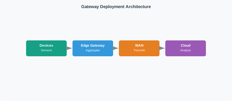
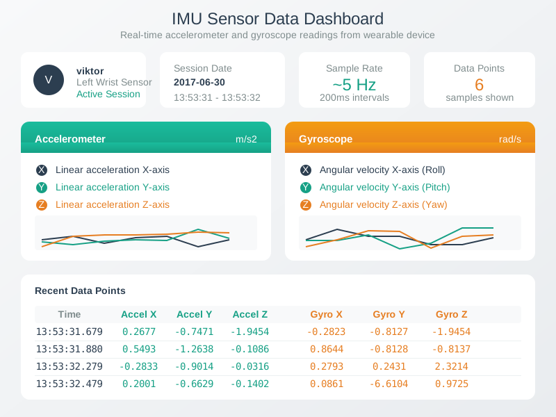
These AI-generated SVG diagrams provide alternative visual perspectives on edge data acquisition concepts covered in this chapter.
Edge Data Acquisition Pipeline
Gateway Deployment Architecture
Accelerometer and Gyroscope Data
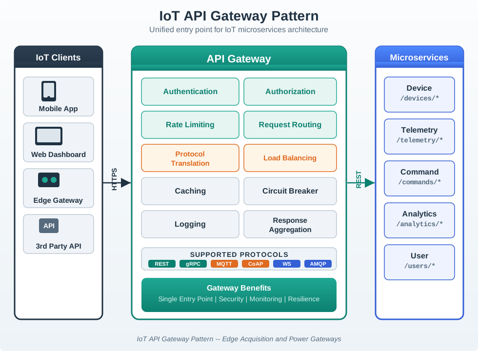
API Gateway Integration
Figure 43.2: AI-generated SVG diagrams illustrating edge data acquisition concepts
43.13 Practice Exercises
Power Budget Battery Exercise
Objective: Calculate battery life for IoT devices with different duty cycling strategies and optimize for maximum longevity.
Tasks:
Select a target device (ESP32 or nRF52): identify power consumption in each state (active sensing: 25 mA, Wi-Fi active: 80-240 mA, light sleep: 0.8 mA, deep sleep: 10 uA)
Calculate average current and battery life with 2500 mAh battery using the formula
Optimize duty cycle: reduce active to 5s/hour, transmit to 2s/hour; recalculate battery life improvement
Expected Outcome: Baseline design yields ~6 months battery life, optimized design achieves 2-3 years (4-5x improvement). Understand that transmission dominates power budget. Learn to batch transmissions and maximize sleep time.
Store-and-Forward Gateway Exercise
Objective: Build a reliable gateway that buffers data during connectivity outages and implements intelligent synchronization.
Tasks:
Set up edge gateway (Raspberry Pi) with local storage (SQLite database or time-series DB)
Implement data pipeline: sensors to gateway (buffer to DB) to cloud (MQTT or HTTP POST)
Add connectivity monitoring: ping cloud endpoint every 10s; if unreachable, set offline flag
Simulate 15-minute outage: disconnect network, accumulate 900 sensor samples (1 sample/sec); reconnect and verify all data syncs with correct timestamps
A small remote-data-logging version can start with a Raspberry Pi reading a DHT22 temperature and humidity sensor, stamping each accepted sample, saving it locally, and then sending the same record to a server or remote machine when the network path is available. Keep the payload boring and auditable: device id, sensor id, temperature, humidity, sample time, quality state, and upload attempt. That record lets the class separate three checks that are often confused in demos: the sensor was read, the gateway kept the reading, and the server received the same timestamped value.
Expected Outcome: Zero data loss during outage with proper temporal ordering after sync. Measure sync latency: 900 records should upload in <10 seconds. Understand buffer sizing: 1 GB storage handles ~10 million sensor readings at 100 bytes each = days of outages.
Key Takeaway
Transmission dominates the power budget of IoT devices. By maximizing deep sleep time and batching transmissions into short bursts, battery life can be extended from months to years. Gateways are essential for bridging non-IP sensors to the cloud, providing protocol translation, store-and-forward buffering, and security – ensuring zero data loss even during network outages.
LoRaWAN Soil Sensor Battery
A precision agriculture deployment uses LoRaWAN soil moisture sensors in vineyards. Target: 3+ year battery life on 2x AA batteries (6600 mAh total @ 3V). Current design lasts only 8 months. Optimize duty cycling to meet requirement.
Initial Design (8-Month Battery Life):
Activity
Duration/Hour
Current Draw
Energy/Hour
Soil moisture sensing (capacitive)
5 seconds
25 mA
0.035 mAh
Temperature sensing (NTC)
2 seconds
3 mA
0.002 mAh
LoRaWAN transmission (SF7, 14 dBm)
2 seconds (packet TX)
120 mA
0.067 mAh
Deep sleep
3591 seconds
50 μA
0.050 mAh
Average current per hour: 0.035 + 0.002 + 0.067 + 0.050 = 0.154 mAh
Battery life: 6600 mAh ÷ 0.154 mAh/hour = 42,857 hours = 4.9 years
Wait - math says 4.9 years, but field deployment lasts only 8 months? What’s wrong?
Root Cause Analysis (Field Measurements):
Actual transmission time: 5 seconds (not 2) due to join/retry overhead
Energy: 5s × 120 mA ÷ 3600 = 0.167 mAh (vs 0.067 planned)
Temperature extremes: Vineyard sees -5°C to +40°C
Battery capacity at -5°C: 6600 × 0.6 = 3960 mAh (40% reduction)
Sleep current higher: Actual measured = 150 μA (not 50 μA)
Cause: ESP32 RTC power domain + LoRa module quiescent current
Actual battery life: 3960 mAh (cold temp) ÷ 0.354 mAh/hour = 11,186 hours = 1.3 years (close to observed 8 months considering further cold-weather losses)
Optimizations to Reach 3+ Years:
Optimization 1 - Reduce Transmission Frequency:
Original: Transmit every hour (24 transmissions/day)
Optimized: Transmit every 4 hours (6 transmissions/day)
Rationale: Soil moisture changes slowly (hourly data unnecessary)
Energy saving: 0.167 mAh/hour × 0.75 = 0.125 mAh/hour saved
Always measure actual field current (don’t trust datasheets for complex sleep modes)
Temperature derating is critical (battery capacity drops 40-60% at freezing)
Transmission dominates power budget - reduce frequency first, then optimize airtime
Store-and-Forward or Cloud
Factor
Direct Cloud Connection (No Gateway)
Edge Gateway with Store-and-Forward
Decision Threshold
Network Reliability
>99% uptime, <10 min/month outage
<95% uptime, hours/day outages
Use gateway if outages >1 hour/week or >0.5% data loss unacceptable
Sensor Protocol
IP-native (Wi-Fi, cellular, Ethernet)
Non-IP (Zigbee, Modbus, BLE, LoRa)
Gateway required for non-IP sensors
Latency Tolerance
Tolerates 1-5 second delays
Needs <100ms local decisions
Use gateway if edge processing required for latency
Data Volume
<1 GB/day per site
>10 GB/day (pre-filter at edge)
Gateway saves bandwidth if raw data >1 GB/day
Security Model
Device-level TLS to cloud
Gateway TLS + device firewall
Use gateway for centralized security policy
Deployment Scale
<100 devices
>1000 devices
Gateway amortizes management cost at scale
Cost per Device
>$50 (justify cellular/Wi-Fi)
<$10 (use low-cost radio)
Gateway enables cheap sensors with radio backhaul
Quick Decision Tree:
Are sensors IP-capable (Wi-Fi/cellular/Ethernet)?
No → Gateway required (protocol translation)
Yes → Continue
Is network connectivity reliable (>99% uptime)?
No → Gateway with store-and-forward (buffer during outages)
Yes → Continue
Is data volume >1 GB/day or real-time processing needed?
Yes → Gateway (edge filtering/processing)
No → Continue
Are there >1000 devices or regulatory security requirements?
Yes → Gateway (centralized management/security)
No → Direct cloud connection (simplest architecture)
Architecture Patterns:
Pattern
When to Use
Example
Direct Cloud
Wi-Fi sensors, reliable network, low volume
Smart home thermostats
Gateway + Store-Forward
Unreliable network, critical data capture
Remote oil pipeline (satellite uplink)
Gateway + Edge Processing
High data volume, need local analytics
Factory vibration monitoring (10 kHz sampling)
Multi-Tier Gateway
Very large scale, hierarchical processing
Smart city (edge → fog → cloud)
Include Transmission Energy
The Error: An engineer designs a wildlife GPS collar using a 3400 mAh battery. Calculation: “GPS module draws 40 mA for 1 minute/hour. Sleep current is 50 μA. Battery life should be 3+ years!” In field testing, collars die after 3 months.
The Flawed Calculation:
Activity
Duration/Hour
Current
Energy/Hour
GPS fix acquisition
60 seconds
40 mA
0.667 mAh
Sleep
3540 seconds
0.05 mA
0.050 mAh
Total
-
-
0.717 mAh/hour
Expected life: 3400 mAh ÷ 0.717 mAh/hour = 4741 hours = 6.6 months (already wrong, but gets worse)
What Was Forgotten - Cellular Transmission:
GPS collars must transmit location to cloud via cellular (2G/3G/4G). Cellular modem characteristics: - Idle (registered to network): 5 mA - Transmitting (GPRS/3G): 200-400 mA peak, 150 mA average - Transmission time: 5-10 seconds per GPS report (TCP handshake + HTTP POST + response)
Revised Calculation:
Activity
Duration/Hour
Current
Energy/Hour
GPS fix
60 seconds
40 mA
0.667 mAh
Cellular TX (10 sec)
10 seconds
200 mA
0.556 mAh
Cellular idle
3530 seconds
5 mA
4.903 mAh
Sleep (GPS/cellular off)
0 seconds
-
0 mAh
Total
-
-
6.126 mAh/hour
Actual battery life: 3400 mAh ÷ 6.126 mAh/hour = 555 hours = 23 days (matches field failure at 3 months with temperature derating + inefficiencies)
Cellular transmission dominated the budget:
GPS: 0.667 mAh (11% of total)
Cellular: 5.459 mAh (89% of total!)
Correct Design - Reduce Transmission:
Option 1 - Batch Transmissions:
Collect 24 GPS fixes in local flash memory
Transmit once per day (1 longer transmission vs 24 short ones)
Cellular modem off 23 hours/day
Activity
Duration/Day
Current
Energy/Day
GPS fix (24x)
24 minutes
40 mA
16 mAh
Cellular TX (1x, 60s)
60 seconds
200 mA
3.33 mAh
Sleep
23.5 hours
50 μA
1.18 mAh
Total/day
-
-
20.51 mAh
New battery life: 3400 mAh ÷ 20.51 mAh/day = 166 days = 5.5 months (still short)
Option 2 - Use Low-Power Radio (LoRaWAN or Satellite IoT):
LoRaWAN transmission: 120 mA for 2 seconds (vs 200 mA for 10 seconds cellular)
No idle current (radio off between transmissions)
Energy: 120 mA × 2s ÷ 3600 = 0.067 mAh per transmission
Activity
Duration/Hour
Current
Energy/Hour
GPS fix
60 seconds
40 mA
0.667 mAh
LoRaWAN TX
2 seconds
120 mA
0.067 mAh
Sleep
3598 seconds
50 μA
0.050 mAh
Total
-
-
0.784 mAh/hour
New battery life: 3400 mAh ÷ 0.784 mAh/hour = 4337 hours = 6.0 months (still needs work)
Option 3 - Combine Batching + LoRaWAN:
GPS fix and transmit every 4 hours instead of hourly (6 cycles/day)
100 mAh/day solar harvest (small 50mm × 50mm panel)
Net drain: 20.51 - 100 = -79.49 mAh/day (battery charges!)
Battery life: Indefinite (solar sustains during daylight, battery covers night)
Key Lessons:
NEVER ignore transmission energy - wireless radios often dominate power budget
Cellular idle current (5 mA) is 100x higher than deep sleep (50 μA) - keep modem off
Batching transmissions reduces overhead (1 long TX < 24 short TXs due to handshake costs)
Low-power radios (LoRaWAN, NB-IoT, satellite IoT) use 50-90% less energy than cellular
Always measure actual field current with ammeter - datasheets lie about sleep current
Checkpoint: Design Tradeoffs
You now know:
A gateway is required for non-IP sensors and valuable when more than 0.5% data loss is unacceptable.
The store-and-forward exercise expects 900 samples from a 15-minute outage to sync in less than 10 seconds.
The design rule repeats: measure field current, reduce transmission frequency, and size buffers for the longest outage.
43.14 Interactive Quiz: Match Concepts
The remaining activities turn the design rules into recall and sequencing checks.
43.15 Interactive Quiz: Sequence the Steps
Common Pitfalls
Budget Transmit Power
Radio transmission is typically the dominant energy consumer in an IoT edge node — often 10x the current draw of the sensor and MCU combined. Any power budget analysis that omits transmission power will dramatically overestimate battery life.
Store-and-Forward Gateways
LoRaWAN, cellular, and Wi-Fi links in remote locations drop regularly. Without local buffering and store-and-forward, every connectivity interruption causes permanent data loss. Size the local buffer for the maximum expected outage duration.
Containerize Gateway Software
A monolithic gateway application that crashes takes down all protocol translation, buffering, and forwarding functions simultaneously. Use containers or process supervisors so individual components can restart independently.
Budget Radio Peak Current
A device’s average current may be 1 mA but its peak during radio transmission may be 200 mA. Under-sized batteries or capacitors that cannot source the peak current will cause voltage drops and resets exactly when data needs to be transmitted.
43.16 Label the Diagram
43.17 Code Challenge
43.18 Radio Budget and Aggregation
The follow-on page narrows the lens to radio scheduling and aggregation contracts.
For the deeper implementation contract behind radio duty cycle, adaptive sampling, gateway aggregation, batching latency, event-preserving summaries, and queue metadata, continue to Radio Budget and Gateway Aggregation Contracts.
43.19 Summary
Power management and gateway functions are critical for practical edge IoT deployments:
Duty cycling: Maximize sleep time and batch transmissions - TX current dominates power budget
Battery life: Optimized duty cycling extends battery life from months to years (4-5x improvement typical)
Gateway functions: Protocol translation, store-and-forward buffering, and security are essential for non-IP device integration
Missing data: Treat as information, not noise - use appropriate imputation and track as a health metric
43.20 Concept Relationships
Power management and gateways are critical constraints that determine edge system feasibility:
Power Optimization (This chapter):
Duty cycling formula extends battery life from months to years (4-5x improvement via deep sleep)
Transmission dominates power budget (10-100x more than sensing); batching is highest-leverage optimization
Key Insight: Power and connectivity are linked – aggressive transmission schedules drain batteries fast. Vineyard case study: Gateways with store-and-forward achieved 0.02% data loss (vs 8% without), while duty cycling achieved 5.4-year battery life (vs target of 3 years). The combination makes low-power, high-reliability IoT feasible.
43.21 What’s Next
If you want to…
Read this
Understand the acquisition architecture this power system supports

 Checkpoint: Duty-Cycle Ledger