28 Feature Scaling and Leakage Controls

28.5 Feature Scales Distort Models

Suppose a model sees temperature in degrees (values around 20) and pressure in pascals (values around 100,000). Many algorithms — anything using distances or gradient descent — will be dominated by the large-magnitude feature purely because of its units, not its importance. Feature scaling puts features on comparable ranges so each contributes on its merits.

The two workhorses are min-max normalisation (rescale to a fixed range like 0 to 1) and z-score standardisation (centre to mean 0, scale to standard deviation 1). Which one to use, and one critical rule about when to compute the scaling, decides whether your model evaluation is honest.

Before choosing a scaler, inspect Figure 28.1 to see where scaling sits in the feature recipe and where leakage can enter. The numbered pipeline separates raw observations, window construction, feature extraction, and normalization, so parameters fitted at the wrong boundary are easier to spot.

Trace Figure 28.1 from raw sensor values through window segmentation and feature extraction to normalized features. Windowing fixes which samples contribute to a training example; extraction gives each feature a physical meaning and unit; normalization changes scale but should not change that meaning. Fit the normalization parameters only on training evidence, then apply the frozen parameters to validation, test, and production data. That order connects scale control to the chapter’s running contract: the deployed feature path must reproduce training without borrowing information from the future or held-out groups.

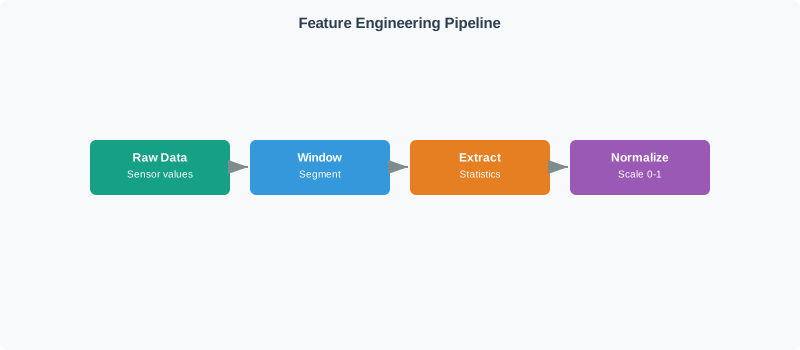
In IoT data this problem appears whenever channels have different engineering units. A room-temperature feature might vary from 18 to 28 degrees C, vibration RMS might vary from 0.02 to 1.5 g, and ambient light might vary from 30 to 90,000 lux. A nearest-neighbour classifier, clustering algorithm, PCA projection, or gradient-based model will treat the lux channel as enormous unless those features are transformed first.

Scaling does not make every feature equally useful. It only removes unit size as a hidden vote. After scaling, the model can still learn that vibration is more predictive than light, but that choice comes from labels and patterns rather than from one sensor reporting larger numbers. This is why normalization belongs after validation and imputation: bad outliers or filled values should be marked before they become training statistics.

The chapter's practical goal is to choose a scaler that fits the feature and the downstream algorithm, then record the parameters used. Without that record, a model trained on scaled inputs cannot be reproduced or served consistently in production.

Overview Knowledge Check

28.6 Min-Max, Z-Score, Robust Scaling

Pick the scaler from the shape of the feature and the model requirement. Min-max scaling is useful when a bounded interval is required, such as a neural-network input expected to sit between 0 and 1. Z-score standardization is the usual starting point for roughly bell-shaped numeric features and distance-based methods. Robust scaling is better when the sensor occasionally sticks, spikes, or produces rare extremes that should not define the whole range.

Always fit the scaler on training data and store the learned parameters. For min-max, that means the training minimum and maximum. For z-score, it means the training mean and standard deviation. For robust scaling, it means the median and interquartile range. Production should apply those saved numbers, not recompute them from each new batch, otherwise the meaning of the model input drifts over time.

Min-max:   x' = (x - min) / (max - min)      -> range [0, 1]; sensitive to outliers
Z-score:   x' = (x - mean) / std             -> mean 0, std 1; the common default
Robust:    x' = (x - median) / IQR           -> resists outliers

Feature stats: min=10, max=50, mean=30, std=8, median=28, IQR=12
A raw value x = 34:

  Min-max:  (34 - 10) / (50 - 10) = 24/40 = 0.60
  Z-score:  (34 - 30) / 8        = 4/8   = 0.50
  Robust:   (34 - 28) / 12       = 6/12  = 0.50

If one wild outlier stretched max to 500, min-max would
squash all normal values near 0. Z-score scaling is also
outlier-sensitive because the mean and standard deviation move;
robust scaling is far less disturbed.

For a small edge pipeline, keep the implementation boring and auditable. Validate the unit and range first, attach quality flags for repaired points, then scale only the numeric features that need it. Do not scale identifiers, categories, timestamps, or binary event labels as if they were continuous measurements. For counters, decide whether the model needs the raw count, a rate, or a log-transformed value before applying a generic scaler.

A simple acceptance check is to print each feature's post-scaling summary: minimum, maximum, mean, standard deviation, missing count, and quality-flag count. If a supposedly z-scored feature has a huge mean, if a min-max feature is mostly pinned at 0 or 1, or if a robust-scaled feature still has unexplained extreme values, the transform is telling you to revisit validation rather than train the model.

Practitioner Knowledge Check

28.7 Fit on Train Only

The most common scaling bug is not the formula; it is the timing. If you split a dataset into train and test, then fit a scaler on the combined data, the training process has already learned something about the test distribution. It may know the future maximum, the future mean, or the future outlier structure. That information is subtle, but it makes evaluation easier than real deployment.

Use this sequence instead: split first, fit the scaler on the training partition, transform the training partition, transform validation and test with the same fitted parameters, then save those parameters with the model artifact. In production, new samples must use that saved scaler. If the production distribution drifts enough that the scaler is no longer appropriate, that is a monitoring event and a retraining decision, not a reason to silently refit the scaler online.

Consider min-max scaling for temperature. Training values range from 18 to 28 degrees C, so 23 degrees C becomes 0.5. If the test set contains a 38 degree overheating event and you fit on all data, 23 degrees C becomes 0.25 instead. The model evaluation now benefits from knowledge that the future maximum exists, and the training representation no longer matches what would have happened before that event was observed.

Some algorithms are mostly scale-invariant, especially decision trees and random forests, because they split on thresholds within one feature at a time. K-nearest neighbours, k-means, PCA, SVMs with distance kernels, linear models with regularization, and neural networks are not. The under-the-hood discipline is to match scaling to the algorithm and keep the scaler as part of the trained system, not as a disposable preprocessing note.

So feature scaling is simple arithmetic with one non-negotiable discipline: fit the scaler on training data alone, persist those parameters, and reapply them unchanged everywhere else. Break that rule and you leak information from the future into the past, producing an invalid estimate that may misstate how the model will perform in the real world.

Under-the-Hood Knowledge Check