29 IoT Worked Examples: Coverage and Decision Tools
More
Depth: Practitioner
Progress saves as you read. Mark sections complete as you go; your progress appears in the sidebar.
- Podcast audio coming soon
- Character narration audio coming soon
29.1 Choose Coverage That Supports a Decision
An IoT network earns its cost when its measurements improve a decision. Nearby sensors can repeat the same information, while a distant gap hides the condition that matters. This chapter connects weather-station spacing, calibration, and investment analysis so that coverage, accuracy, and cost can be judged together. It is part 2 of 2; IoT Worked Examples: Deployment Economics supplies the earlier cases.
A regional agricultural extension service needs automated weather observations for precision farming across 12,000 km². Its 2,400 farms average 500 hectares each, but coastal, valley, and upland terrain behave differently. Farmers need frost warnings, irrigation guidance, and disease prevention. A uniform network may spend money repeating coastal readings while missing an upland frost pocket.
The problem is to choose enough useful observation sites within a budget, then show what evidence supports the claimed benefit. We will first examine a terrain-aware weather design, compare it with four other deployments, and connect the financial terms. Then we will use separate decision tools and a municipal example to test the assumptions behind a promising return.
KEY CONCEPTS
- Useful coverage
Terrain and critical locations determine where observations matter.
- Calibration hierarchy
Reference measurements anchor cheaper coverage sensors.
- Lifecycle cost
Capital and recurring costs both shape the investment case.
- Realized benefit
Adoption and rollout determine when projected value arrives.
29.2 Learning Objectives
By the end of this chapter, you will be able to:
- choose weather-station spacing from coverage evidence
- compare cost, coverage, and accuracy across examples
- use calibration, network, and ROI tools with stated limits
29.3 Place Weather Stations Around Terrain
The extension service’s coastal zone covers 3,000 km², the valley 4,000 km², and the uplands 5,000 km². Its stated frost requirement combines 95% detection with temperature accuracy within ±1.5°C. The budget allows $180,000 in capital and $28,000 per year for operations; each full weather station costs $8,500. Coverage therefore has to be selective without quietly relaxing the frost target.
A correlation distance describes how far apart points can be while retaining similar measurements. In this example, coastal temperature remains predictable over 22 km. In mountainous uplands, conditions in a valley 6 km away may differ substantially. Shorter correlation distances require more observation sites per square kilometer, and the relevant distance depends on the measurement as well as the terrain.
The worked coverage estimates are eight full stations for flat coastal terrain at 22 km correlation distance, 36 for moderately complex valley terrain at 12 km, and 177 for complex uplands at 6 km. These are supplied placement estimates, rather than counts derived from correlation distance alone. Their sum is 221 stations; the upland requirement by itself already exceeds the capital budget.
The proposed hybrid instead places full stations at 12 key upland sites, adds 30 temperature-only loggers at $350 each for frost monitoring, and uses elevation-based interpolation between stations. Interpolation estimates conditions in the gaps from observed sites and elevation. It is the assumption that makes the smaller network plausible; a temperature logger does not replace a full station’s multiple weather measurements.
The final proposal has 21 full stations and 30 loggers, or 51 observation devices. Its hardware arithmetic is:
21 × $8,500 + 30 × $350 = $189,000.
That is $9,000 above the $180,000 capital limit. The design needs an approved increase or revision before it can be presented as affordable. The source does not allocate all remaining full stations between the coastal and valley zones, so those placements also need an explicit design record.
The worked temperature result is a root mean square error (RMSE), a measure of prediction error, of 1.2°C. It is below the stated 1.5°C threshold, but an average error does not establish that every prediction lies within ±1.5°C. The 97.3% frost-detection figure is a simulated assumption, pending held-out observations across zones and seasons. Meeting an error threshold in a model and demonstrating the 95% detection target in operation are separate validation tasks.
Validation must therefore preserve the purpose of each observation. Full stations supply the weather reference, while the additional loggers strengthen frost monitoring between them. Check whether the interpolation remains useful in each topographic zone and season before relying on the aggregate result. The key question is whether the sparse observations support the alert decision at the farms that would otherwise fall between full stations.
The modeled annual farmer benefit combines $504,000 of prevented frost damage, $340,000 of irrigation water savings, and $180,000 of disease prevention: $1.024 million per year. If the additional capital is approved, $189,000 ÷ $1.024 million × 12 gives about 2.2 months of gross-benefit payback. That arithmetic precedes operating-cost, adoption, and rollout adjustments.
A cost comparison also needs a named baseline. Against the separately stated uniform baseline of 225 full stations, hardware would cost 225 × $8,500 = $1.9125 million. The $189,000 hybrid is about 9.9% of that amount, rather than the earlier 35% claim. The 225-station baseline differs from the 221 total in the zone estimates; preserve that distinction when reviewing the comparison rather than treating them as one calculation.
29.4 Compare Placement Patterns Before Ranking Returns
The weather proposal becomes more useful when compared with the other four worked examples. Their domains and scales differ, so a device count alone cannot explain their value. Application Domains provides the wider domain context; here the question is how each deployment connects locations to decisions.
The portfolio figure compares counts and financial assumptions. Read its placement patterns before using any payback ranking, and use the figures in the text below where a rounded comparison obscures an important qualification.
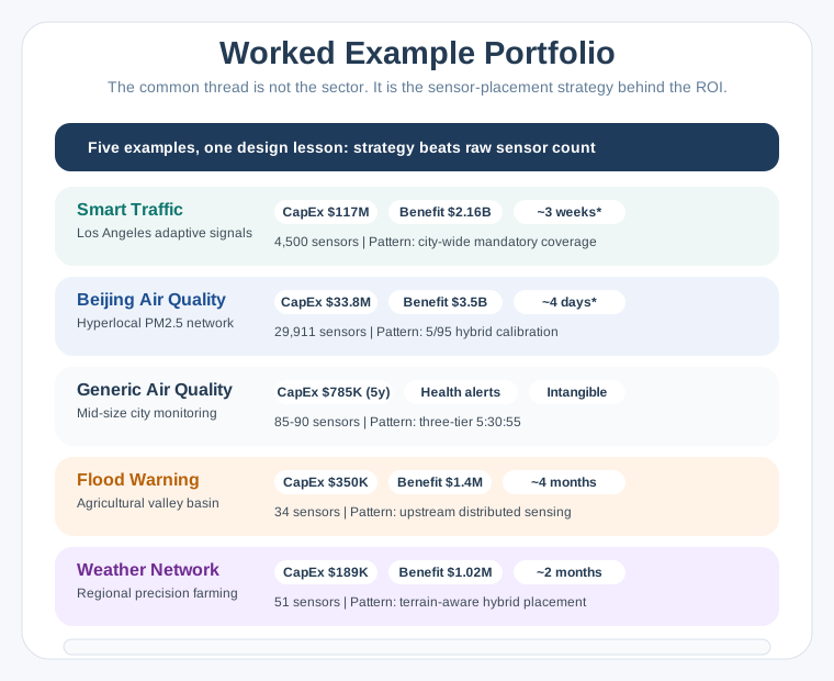
- Smart traffic in Los Angeles: $117 million capital expenditure, $2.16 billion annual benefit, about three weeks theoretical payback, and 4,500 intersections requiring city-wide deployment.
- Air quality in Beijing: $33.8 million capital expenditure, $3.5 billion annual benefit, about four days theoretical payback, 29,911 sensors, and a 5/95 reference-to-low-cost hybrid calibration mix.
- Generic air quality: $817,100 five-year cost for 85 stations, still over budget, or $799,720 for the separately costed 74-station option. The tier counts are 5:30:50 before that additional cut.
- Flood warning: $350,000 capital expenditure, $1.4 million annual benefit, about four months payback, 34 sensors, and upstream distributed sensing.
- Weather network: $189,000 capital expenditure, approximately $1.02 million annual benefit, about two months gross-benefit payback, and 51 stations or loggers placed around terrain.
Beijing has almost thirty thousand devices; flood warning has thirty-four. Their payback estimates do not rank by sensor count. What differs is the placement pattern: every intersection, a few reference stations supporting many cheaper sensors, a three-tier mix, upstream sensing, or terrain-aware weather sites. The flood case’s upstream rain and river data creates a stated 6–10-hour warning lead time. Its historical damage baseline and warning-to-action link also make avoided losses comparatively measurable, although attribution still needs evidence.
Traffic and air-quality examples show that full coverage at lower precision can beat partial coverage at high precision.
Starred portfolio paybacks assume the entire network switches on at once. The traffic calculation’s 19.7-day result makes that assumption for all 4,500 intersections. A deployment ramp delays benefit; model the installation schedule and benefit curve rather than applying a universal 3–5× payback multiplier. Neither a universal 12–24-month deployment nor an 18–30-month payback follows from these examples.
The comparison also separates benefits that are easy to state from benefits that can be attributed to a network. Large projected traffic or health savings still need a link from measurement to action to realized outcome. The weather service faces the same issue: estimating frost damage is different from showing how much damage its warnings prevented. Use the portfolio to identify the evidence each case needs.
29.5 Connect Coverage Evidence to the Business Case
Placement creates value only when its observations support action. The Three Ingredients Test and Five Verbs Framework help describe that connection. The eleven ideal IoT characteristics then help turn an attractive pattern into requirements that can be checked.
Capital expenditure (CapEx) covers hardware, installation labor, and software licenses. Professional installation can materially increase cost, so estimate site access, labor, commissioning, and local rates. Operating expenditure (OpEx) covers recurring connectivity, maintenance, cloud services, and staff. Over five years it often equals or exceeds capital cost. Total cost of ownership (TCO) combines these costs over the chosen lifecycle.
A tiered sensor strategy matches measurement quality to location criticality. A calibration hierarchy uses reference measurements to assess and correct cheaper sensors. Reference instruments are chosen around regulatory and measurement-uncertainty needs; an illustrative 5–10% of the fleet can carry much of the data-quality burden. That percentage is a starting hypothesis, not a substitute for local validation.
Adoption rate is the share of intended use actually achieved. Behavior, technology access, and training determine how much theoretical benefit becomes realized benefit. The examples use 15–30% sensitivities, and a matching activity uses 10–30%; neither range is a universal forecast. In the Beijing model, an assumed $17.4 billion maximum multiplied by 15% uptake gives $2.61 billion. This is a scenario sensitivity, separate from the portfolio’s $3.5 billion benefit estimate and from any measured outcome.
Payback period describes how long net benefit takes to recover capital spending. Return on investment (ROI) compares benefit after costs with the investment. A comparative case must include lifecycle costs; discounted analysis also states the discount rate. Simple payback and undiscounted five-year ROI do not themselves account for the time value of money.
Build the case in a connected sequence: identify a measurable benefit, choose critical sites and sensor tiers, calculate capital and operating costs, apply a project-specific adoption forecast, and calculate payback from the deployment timeline. Evaluate the return over a 5–10-year lifecycle, with five-year TCO visible. A high count or positive dashboard return cannot replace calibration, coverage, and local financial evidence.
Keep the financial record connected to the coverage record. A reduction in the number of sites may lower capital cost while changing the geography served; a reduced operating allowance may change maintenance or calibration. Revisit the benefit estimate when either design changes. Otherwise, the cost calculation describes one network while the benefit calculation silently assumes another.
29.6 Use the Network Designer to Expose Assumptions
With the framework explicit, the separate network designer lets you vary coverage, terrain, costs, and budget. Its inputs are rehearsal assumptions, not vendor quotes. Set the total area in km², choose terrain complexity, replace sensor prices with local quotes, and inspect both cost and the resulting coverage.
The calculator uses correlation distances of 20 km for flat terrain, 12 km for moderate terrain, and 6 km for complex terrain. Its flat-terrain assumption differs from the weather case’s 22 km. Under its simple area-density model, moving from 20 km to 6 km implies about 11 times as many sites. That explains the sensitivity to terrain without proving that either spacing is locally adequate.
Treat the 5/30/65 reference/mid-grade/low-cost mix as a selectable starting design whose accuracy needs validation. The calculator retains at least three reference sensors for calibration redundancy; this is a model constraint, not a universal minimum. Its illustrative 75–90% savings against all-reference deployment depend on the sensor prices and baseline. Budget-driven reductions in sensor count change the coverage proposition and must be reviewed as a revised design.
Observe where shorter correlation distance increases count, where lower-cost tiers reduce expenditure, and whether reference anchors remain sufficient. A cheaper mix is useful only if calibration supports the intended decisions. The broader two-tier examples use 5–10% reference instruments and 90–95% cheaper coverage; the three-tier example instead suggests 5–10% reference, 30–40% mid-grade, and 50–60% low-cost. These are different example mixes, not interchangeable guarantees.
This is why the designer should be read as a comparison tool. First compare the same area under different terrain assumptions, then compare sensor mixes under the same coverage assumption. If a budget adjustment removes sites, return to the placement decision before accepting the revised total. Maintaining calibration anchors and meeting the budget are necessary checks, but neither alone demonstrates adequate spatial coverage.
29.7 Use the ROI Tool to Test Timing and Uptake
Coverage assumptions feed the separate ROI calculator. Select Smart Traffic, Air Quality, Flood Warning, Weather Network, or Custom, then adjust capital cost, annual operating cost, gross benefit, adoption, and deployment months. The tool displays payback, ROI, and viability as those inputs change.
The core relationship is annual net benefit = gross annual benefit × adoption rate − annual OpEx. Equal capital spending does not imply equal payback when operating costs differ. The separate check compares two $500,000 projects with $200,000 gross annual benefit and different operating bills to make that dependency visible.
The tool’s screening guidance flags payback above three years, OpEx above 20% of CapEx annually, and adoption below 15%. Those prompts respectively suggest reviewing funding expectations, recurring costs, and training or change management. A 3:1 benefit-cost ratio is presented as a strong-project signal, but the ratio’s denominator matters: the current tool compares annual adoption-adjusted benefit with annual OpEx, rather than total lifecycle cost.
The calculator also adds deployment months to steady-state payback as a simple timing approximation. Do not present that output as a complete cash-flow model: commissioning schedules determine when partial benefits begin. Likewise, its five-year ROI is a simplified undiscounted calculation. Watch how adoption changes net benefit, distinguish theoretical from project-start payback, and inspect the assumptions behind any favorable display.
29.8 Read the Parking Arithmetic as a Conditional Case
The parking example puts the same framework into a complete calculation. A city of 250,000 people considers 800 spaces in 12 multi-level downtown garages. The scenario assumes availability information saves eight minutes of circling per parker. It values driver time at $27 per hour and fuel savings at $0.85 per avoided circling event. These inputs describe the modeled benefit; they do not establish that every parker uses the service.
Hardware costs are $125 per space sensor and $2,400 per gateway, with one gateway per garage. Installation is $45 per sensor. Capital cost therefore combines 800 × $125 = $100,000 for sensors, 12 × $2,400 = $28,800 for gateways, and 800 × $45 = $36,000 for installation, totaling $164,800.
Annual operations include $8 per month of cellular connectivity per gateway, a $15,000 cloud platform, and a 12% annual sensor-failure assumption. Connectivity is 12 × $8 × 12 = $1,152; replacement hardware is 800 × 12% × $125 = $12,000. Together with cloud service, annual OpEx is $28,152, approximately 17% of CapEx.
The scenario has 2,400 daily parkers on 260 workdays and 1,800 on 105 weekend days. At eight minutes each, workday time savings are 83,200 hours and weekend savings 25,200 hours. The total 108,400 hours × $27 = $2,926,800 annual time value. The same attendance assumptions give 813,000 annual parking events, producing $691,050 of fuel savings at $0.85 each.
Total modeled annual benefit is $3,617,850. Subtracting $28,152 OpEx gives $3,589,698 annual net benefit, and $164,800 ÷ $3,589,698 gives 0.046 years, or about 17 days, of theoretical payback. A daily problem affecting thousands of users can produce a large modeled return, but the result is conditional on the savings, use, coverage, and timing assumptions.
Read the parking result in that order: physical deployment, recurring service, assumed changes in driver behavior, then financial return. All twelve garages contribute to the full-coverage calculation. If only half are deployed, the original benefit cannot simply remain attached to the smaller project. The question is which parking events receive useful availability information and how the changed coverage affects the assumed time and fuel savings.
Five-year TCO is $164,800 + 5 × $28,152 = $305,560. Five years of modeled gross benefit is approximately $18.089 million, giving a gross benefit-to-cost multiple of about 59×. That multiple is not ROI: ROI also subtracts costs, and a realistic case requires adoption assumptions. The separate exercise asks how the case changes with only six of twelve garages covered, what share of five-year costs is recurring, and whether the three-year municipal funding screen is met.
29.9 Replace Uniform Density With Useful Measurements
The final municipal example shows why a large purchase can still miss the decision. This is a fictional air-quality network exercise. Its population, zones, sensor performance, audit findings, and before/after outcomes are assumed inputs, rather than evidence from a named city audit.
The fictional city has 600,000 residents and installs 200 identical $800 sensors on a 1 km uniform grid. Hardware costs $160,000, installation $40,000, and five-year connectivity $60,000, for $260,000 total investment. The imagined audit occurs after 18 months. Three industrial zones occupy 12% of the area but account for an assumed 65% of pollution; their hotspots are undersampled, while 88 residential sensors largely repeat low-variability readings.
All 200 devices are the same low-cost model, with no reference-grade calibration anchors. The exercise assumes 15–30% drift over 12 months, about 60 useful sensors (30% utilization), and measurement error around ±25% against a ±10% target. It also assumes missed critical sites at 18 schools, four hospitals, and eight highway corridors, three policy decisions later reversed, and loss of council confidence in the smart-city program.
A proposed replacement uses eight $15,000 reference sensors ($120,000) at industrial boundaries for calibration anchors and regulatory needs, 30 $3,000 mid-grade sensors ($90,000) at schools, hospitals, highways, and industrial fence-lines, and 50 $800 low-cost sensors ($40,000) for residential coverage. That is 88 sensors and $250,000 of hardware, or 56% fewer devices. Reference measurements anchor quality, critical sites receive better instruments, and cheaper sensors fill spatial gaps with calibration against nearby Tier 1/2 measurements.
The replacement’s hardware alone costs more than the original $160,000 hardware bill. Its $250,000 is not a complete replacement lifecycle budget comparable with the original $260,000 investment; installation and recurring costs still need costing. A lower count does not establish either an affordable redesign or decision-grade accuracy.
The assumed three-year comparison takes useful devices from about 60 to all 88, error from about ±25% to maintained ±8%, and critical-site coverage from 0% to 100%. It changes three reversed policy decisions to 14 validated decisions and a data-quality rating from 2.1/5.0 to 4.4/5.0. Hardware cost per useful sensor rises slightly, from $2,667 to $2,841. These fictional outcomes illustrate what to measure; sensor tiers alone do not prove those improvements.
For a real deployment, identify 10–20 critical locations with meteorologists, urban planners, and public-health experts before filling gaps. Install reference instruments in Month 1 of the example rollout and calibrate cheaper nodes before relying on their data. Set the actual number of anchors from uncertainty and regulatory needs. Strategic placement can outperform a uniform grid, while sufficient coverage remains necessary.
The separate check also revisits a $200,000 choice: 250 identical $800 devices versus five $15,000 reference units, 30 $3,000 mid-grade units, and 50 $800 coverage units. The latter totals 85 sensors but $205,000, so calibration advantages do not make it fit the stated budget. Both placement evidence and complete arithmetic belong in the approval decision.
Summary
Useful coverage follows terrain, critical locations, and the decision being supported. The weather case combines full stations, temperature loggers, and interpolation; its $189,000 hardware cost exceeds budget, and its simulated frost performance still needs validation. Across the five examples, placement patterns explain more than device count alone.
A defensible business case quantifies capital cost, recurring cost, and measurable benefit together. It discounts theoretical benefits with a project-specific adoption forecast, includes five-year TCO, and follows the rollout from project start. The parking arithmetic and fictional municipal redesign show why impressive returns and lower sensor counts still require evidence. Use the Quiz Navigator to revisit these ideas across chapters.
Place sensors where they improve decisions, validate the cheaper coverage layer, and calculate returns from complete costs and benefits that users can actually realize.
Next, Common Pitfalls examines the mismatches that can undermine an otherwise promising IoT project.