28 IoT Deployment Economics: Rollout and ROI Evidence
More
Depth: Practitioner
Progress saves as you read. Mark sections complete as you go; your progress appears in the sidebar.
- Podcast audio coming soon
- Character narration audio coming soon
28.1 From a rollout budget to evidence
A deployment budget tells a city what it must spend. A return on investment, or ROI, claim also needs evidence that coverage, adoption, and timely action produce the expected benefit. This second part follows IoT Deployment Economics: Budget Models, using its traffic upgrade before examining air-quality and flood-warning networks in the applications module.
Start with the city’s 4,500-intersection traffic upgrade. A small corridor can be installed before the rest of the network, but shared costs may arrive before network benefits. Even a technically working pilot leaves two questions: what happens outside its boundary, and when do residents begin receiving the modeled benefit?
That is the partial-deployment problem. Stage gates—decisions about whether to continue a rollout—must test adoption and benefit before scale. The approaches below connect phased coverage to benefit timing, use calibrated sensor tiers to separate coverage from measurement quality, and place flood sensors where they provide enough time to act.
KEY CONCEPTS
- Coverage
A pilot boundary can hide costs and effects outside it.
- Calibration
Reference sensors anchor the cheaper coverage layer.
- Adoption
Potential benefit depends on people using the service.
- Warning time
Upstream evidence must arrive early enough for action.
28.2 Learning Objectives
- Identify the partial-deployment trap in an IoT business case.
- Test ROI claims with rollout and sensitivity evidence.
28.3 Test the rollout boundary and benefit timing
A corridor of 50–100 smart intersections can shift traffic toward adjacent non-smart signals and create new bottlenecks. Treat these effects as part of the pilot’s evidence. The source’s Pittsburgh Surtrac example motivates coordinated coverage, but does not establish that city-wide deployment is a universal technical requirement. Budget for phased coverage in Phase 1 and measure effects at adjacent signals before extending the claim to the whole city.
Keep the time-saving arithmetic separate from the rollout schedule. With 800,000 commuters, a 28-minute one-way commute, 250 days per year, and a 10% reduction, each commuter saves 2.8 minutes one way per day. The total is about 9.33 million driver-hours per year. At $25 per driver-hour, the annual value is approximately $233 million. This is a one-way calculation; its benefit depends on delivering the assumed reduction.
The preceding worked example’s 19.7-day simple payback assumes full benefits begin immediately. Installing 4,500 intersections instead takes an assumed 12–24 months, with modeled payback around 18–30 months after project start as benefits ramp up. A division can be arithmetically correct while its timing assumption fails. Now apply that distinction between modeled potential and delivered benefit to an air-quality network.
28.4 Build the Beijing coverage and benefit case
The Beijing network combines reference-grade sensors with a larger low-cost layer to support local air-quality decisions. Reference sensors provide calibration evidence for the cheaper devices rather than replacing their spatial coverage. The budget includes installation, connectivity, and platform costs as well as sensor purchases. The benefit model discounts potential value by adoption because residents must use the routing service for its proposed benefit to occur.
Hypothetical planning scenario: Model a hyperlocal air quality monitoring network for Beijing, China (population 21,540,000) to provide block-level PM2.5 alerts and enable pollution-responsive traffic routing. The sensor counts and costs below are modeled assumptions, not observed deployment figures.
The planning inputs make the scale and price assumptions explicit:
- City area: 16,411 km^2
- Population density varies: 1,200/km2 (suburbs) to 45,000/km2 (urban core)
- Target resolution: 250 m urban grid; the detailed plan uses a 500 m suburban ring and a 1 km outer-area grid
- Reference-grade sensor cost: $12,500 each (meets regulatory standards)
- Low-cost sensor cost: $385 each (requires calibration against reference)
- Data transmission: NB-IoT at $2.50/month/sensor
- Health cost of PM2.5 (fine particulate matter): assumed $95 per µg/m³ per person per year (attributed to WHO in the source; no supporting citation is supplied)
Work from spatial coverage to the purchase bill, recurring costs, and only then the benefit claim:
-
Calculate sensor density requirements:
- Urban core (500 km^2): 250m grid = 16 sensors/km^2 = 8,000 sensors
- Suburban ring (2,000 km^2): 500m grid = 4 sensors/km^2 = 8,000 sensors
- Outer areas (13,911 km^2): 1km grid = 1 sensor/km^2 = 13,911 sensors
- Total sensors needed: 29,911 sensors
-
Design hybrid sensor network:
- Reference-grade (5% of network): 1,496 sensors x $12,500 = $18.7M
- Low-cost (95% of network): 28,415 sensors x $385 = $10.94M
- Installation and mounting: $45 x 29,911 = $1.35M
- Central platform and analytics: $2.8M
- Total capital expenditure (CapEx): $33.79M
-
Calculate annual operating costs:
- NB-IoT connectivity: 29,911 x $2.50 x 12 = $897K/year
- Sensor replacement (15% annual): 4,487 sensors x $450 avg = $2.02M/year
- Calibration technicians (25 FTE): $625K/year
- Cloud processing and storage: $1.2M/year
- Total operating expenditure (OpEx): $4.74M/year
-
Calculate pollution reduction from routing:
- Assume traffic contributes 35% of PM2.5 in this Beijing planning scenario.
- Assume dynamic routing reduces exposure in hotspots by 22%.
- Assumed illustrative population-weighted exposure reduction: 8.5 ug/m^3 average; the inputs above do not derive this value
- Health benefit: 21.54M people x $95 x 8.5 = $17.4B/year potential
- Achievable benefit (15% of population uses routing): $2.61B/year
-
Calculate alert system value:
- High-pollution days: 127/year average
- Vulnerable population (children, elderly, respiratory conditions): 4.8M
- Assume an alert adoption rate of 45% checking daily readings.
- Assume 12% exposure is avoided through behavior change on alert days.
- Assumed illustrative health savings: $890M/year; the stated inputs do not derive this value
-
Calculate ROI:
- Total annual benefit: $2.61B + $890M = $3.5B
- Net benefit: $3.5B - $4.74M = $3.495B/year
- Payback period: $33.79M / $3.495B = 3.5 days
- Benefit-cost ratio: about 431:1 over 10 years (undiscounted)
Result: Hyperlocal air quality network investment of $34M generates $3.5B annual health benefit in the scenario. The hybrid sensor approach (5% reference-grade, 95% low-cost) reduces sensor hardware cost by about 92% against an all-reference purchase; calibration performance must be verified separately.
These large modeled returns depend on the assumed exposure reduction and uptake. City-average readings can miss pollution hotspots, so prioritize dense sensing in high-population, high-pollution corridors. Test calibration, routing adoption, and exposure changes before treating the $3.5 billion as a delivered annual health benefit. The 3.5-day quotient is a steady-state calculation, subject to the same benefit-ramp problem as traffic signals. The alert assumptions also need validation before the $890 million can be accepted.
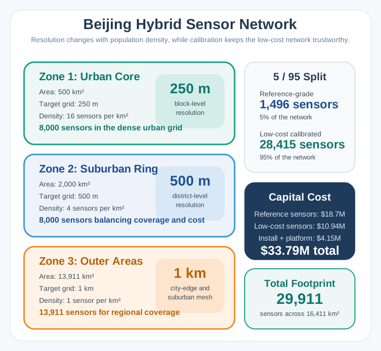
Read Figure 1 from the dense core to the outer area. The core needs 500 km² × 16 sensors/km² = 8,000 sensors; the suburban ring adds another 8,000, and the outer 13,911 km² adds 13,911. The total is 29,911 sensors. A 5% reference-grade share calibrates the 95% low-cost estate: 1,496 reference units plus 28,415 low-cost units. Their $29.64 million equipment cost, about $1.35 million installation, and $2.8 million platform sum to the shown $33.79 million capital estimate.
28.5 Preserve calibration while buying coverage
The Beijing 5/95 split is a hybrid sensor network: reference-grade instruments supply calibration evidence for a larger inexpensive coverage layer. Its approximately 92% hardware saving is relative to an all-reference purchase, not a guarantee of data quality sufficient for health advisories. At $12,500 for each of 29,911 locations, all-reference hardware would cost $373,887,500, or about $374 million, against the hybrid equipment bill of $29.64 million.
28.6 Tiered Sensor Economics
A smaller 100-sensor comparison makes the same distinction with different unit prices. All-reference hardware costs 100 × $5,000 = $500,000. A 5:95 tiered purchase costs (5 × $5,000) + (95 × $300) = $25,000 + $28,500 = $53,500. The saving, ($500,000 − $53,500) / $500,000, is approximately 89%. The 89% and 92% results belong to their respective price assumptions.
In this worked comparison, reference sensors calibrate low-cost units every 6 hours, correcting drift and maintaining correlation r > 0.85 with EPA-grade instruments. Treat that performance as a condition to verify separately before adopting the network. The reference layer corrects drift and bias; removing it changes the evidence behind the inexpensive readings as well as the bill. Neither calibration nor a low hardware price establishes that residents will use the routing app.
The pattern also appears in water quality, noise monitoring, and soil analysis. Reference sensors act as “truth anchors” for the wider network. The next budget makes the placement tradeoff sharper: which coverage can be reduced while preserving those anchors and evidence at critical locations?
28.7 Urban Air Quality Network Design
The smaller urban design assigns reference units to calibration, mid-grade units to critical locations, and inexpensive units to spatial density. Preserve those roles when reviewing cuts: reducing the coverage tier changes spatial detail while retaining calibration anchors and critical-location evidence.
Scenario: A city of 500,000 residents is deploying a hyperlocal air quality monitoring network to identify pollution hotspots, support public health advisories, and evaluate the effectiveness of low-emission zones.
The monitoring responsibilities and budget are:
- City area: 150 km^2 (urban core: 50 km^2, suburban: 100 km^2)
- Population density: Urban core 8,000/km^2, suburban 1,000/km^2
- Major pollution sources: 3 industrial zones, 15 major intersections, 1 port
- Air quality parameters: PM2.5, PM10, NO2, O3, CO, temperature, humidity
- Regulatory requirement: Data resolution sufficient to trigger health alerts at neighborhood level
- Budget: $800,000 for 5-year deployment (capital + operations)
Assign locations first, then cost the tiers and their support over five years:
-
Determine spatial resolution requirements: For this example, plan a 1 km urban grid and a 2 km suburban grid, adding 500 m coverage at priority hotspots after checking local siting and calibration needs.
- Urban core (50 km2): 1 km grid = 50 reference points, plus 20 high-priority locations = 70 locations
- Suburban (100 km^2): 2 km grid = 25 reference points
- Total monitoring locations: 95
-
Select sensor tiers based on location criticality:
- Tier 1 (Reference-grade, $15,000 each): 5 units for regulatory compliance and calibration
- Tier 2 (Mid-grade, $3,000 each): 30 units at industrial boundaries, major roads, schools
- Tier 3 (Low-cost indicative, $800 each): 50 units for spatial coverage
- Sensor costs: (5 x $15,000) + (30 x $3,000) + (50 x $800) = $75,000 + $90,000 + $40,000 = $205,000
-
Calculate connectivity costs (5-year):
- Tier 1/2 sensors (cellular, high reliability): 35 x $15/month x 60 months = $31,500
- Tier 3 sensors (LoRaWAN): 50 x $3/month x 60 months = $9,000
- LoRaWAN gateways (8 needed for coverage): 8 x $1,200 = $9,600
- Total connectivity: $50,100
-
Infrastructure and installation:
- Mounting hardware and enclosures: 85 x $400 = $34,000
- Professional installation (Tier 1/2): 35 x $800 = $28,000
- Community installation (Tier 3): 50 x $200 = $10,000
- Total installation: $72,000
-
Operations and maintenance (5-year):
- Calibration visits (Tier 1 quarterly, Tier 2 semi-annual): $120,000
- Sensor replacement (20% failure rate over 5 years): $45,000
- Data platform and analytics: $150,000
- Staff (0.5 FTE technician): $175,000
- Total operations: $490,000
-
Budget validation:
- Total 5-year cost: $205,000 + $50,100 + $72,000 + $490,000 = $817,100
- The 85-station network remains $17,100 over budget.
- If the $800,000 cap is binding, reduce Tier 3 by 11 more units (from 50 to 39): each removed unit saves $1,580 over five years ($800 sensor + $180 connectivity + $600 mounting/installation), so the 74-station option costs $799,720. Recheck spatial coverage before adopting it.
Result: The 85-station option remains over budget. A separately costed 74-station option is within the cap but needs a spatial-coverage review before adoption.
The decision is therefore explicit: Urban air quality networks require a tiered sensor strategy. A few expensive reference-grade sensors provide accuracy anchors for calibrating many lower-cost sensors. The 5:30:50 ratio (reference:mid-grade:low-cost) balances spatial coverage with data quality in the 85-station option, which exceeds this example’s budget by $17,100.
If funding falls by 30%, review low-cost Tier 3 coverage first while preserving scarce reference anchors and the mid-grade layer. A proportional cut across all tiers would also weaken calibration. Any cut still needs a coverage review: the original spatial requirement names 95 monitoring locations, while the costed options supply only 85 or 74 stations. Neither option by itself demonstrates that every required location is served.
28.8 Compare costs on the same basis
The two air-quality plans address the same coverage-and-calibration problem at different scales. Keep the cost horizon visible when comparing them.
| Planning measure | Hypothetical Beijing plan | Generic city plan |
|---|---|---|
| Sensors | 29,911 | 85 over budget; 74 within cap |
| Tiers | Reference and low-cost | Reference, mid-grade, low-cost |
| Grid resolution | 250 m to 1 km | 500 m hotspots to 2 km |
| Connectivity | Uniform NB-IoT | Cellular and LoRaWAN |
| Capital estimate | $33.79M | Included in the five-year totals below |
| Five-year cost | $57.49M at stated annual OpEx | $817,100 for 85; $799,720 for 74 |
Beijing’s $33.79 million is capital expenditure, not a five-year total. Adding five years at $4.74 million gives $57.49 million before discounting. The generic city’s $817,100 and $799,720 already include five-year operations, so comparing either directly with Beijing’s capital figure would mix cost bases.
The source’s near-$1.57-per-resident comparison likewise mixes horizons. Beijing capital is about $1.57 per resident; its five-year total is about $2.67. The generic options cost about $1.63 and $1.60 per resident over five years. The populations differ by about 43 times (roughly the source’s 40× comparison), while sensor counts do not scale proportionally. Treat the source’s $1.50–$2.00 heuristic as an illustrative figure requiring a stated horizon and coverage requirement, rather than a transferable municipal budget rule.
Both air-quality cases show that buying sensors is only one step toward useful action. Flood warning makes the next constraint unavoidable: a measurement can be accurate and connected yet arrive too late to protect anyone.
28.9 Flood Early Warning Network
Scenario: A regional water authority is deploying an IoT-based flood early warning system for a 200 km river basin that includes 15,000 hectares of farmland, 3 towns (combined population 45,000), and critical infrastructure.
The authority must meet these action windows with the available infrastructure:
- River length: 85 km from headwaters to valley floor
- Catchment area: 1,200 km^2
- Warning time needed: 4 hours minimum for evacuation, 8 hours for livestock relocation
- Existing infrastructure: 2 manual river gauges (read daily), 1 weather station
- Budget: $350,000 capital, $40,000/year operations
Follow the hazard from headwaters to valley floor when assigning sensors and support costs:
-
Map sensor requirements by zone:
- Upper catchment (headwaters to km 30): 8 rain gauges + 4 stream level sensors
- Mid-catchment (km 30-60): 6 river level sensors + 4 soil moisture sensors
- Lower catchment (km 60-85): 8 river level sensors + 4 flood extent sensors
- Total sensors: 34
-
Select appropriate sensor technologies:
- Rain gauges (tipping bucket): 8 x $1,200 = $9,600
- Stream/river level (radar or ultrasonic): 18 x $2,500 = $45,000
- Soil moisture (capacitive): 4 x $400 = $1,600
- Flood extent (pressure transducer): 4 x $800 = $3,200
- Total sensors: $59,400
-
Design connectivity architecture:
- Upper catchment (no cellular): Satellite connectivity
- Mid/lower catchment: LTE-M cellular
- 5-year connectivity cost: $41,460
-
Implement prediction and alerting system:
- Hydrological model calibration: $45,000
- Edge computing at central hub: $12,000
- Alert system (SMS, sirens, radio integration): $35,000
- Mobile app development: $25,000
- Total software/alerting: $117,000
-
Installation and infrastructure:
- Solar power systems (upper catchment): $9,600
- Mounting structures: $20,400
- Professional installation: $45,000
- Total installation: $75,000
-
Calculate flood damage prevention value:
- Average annual flood damage: $2.8 million
- Damage reduction with 4-hour warning: 40-60%
- Expected annual savings: $1.1-1.7 million
- Simple payback: approximately 3–4 months on an annualized avoided-damage basis
Result: 34-sensor flood warning network providing 6-10 hour advance warning for valley communities.
The placement decision follows the warning requirement: Flood early warning systems require sensors distributed across the ENTIRE catchment, not just at the point of interest. Upper catchment rainfall data provides the critical 6-10 hour lead time needed for effective response.
Rain in the upper catchment causes flooding in the lower valley 6–10 hours later. Place sensors where that process begins to gain warning time.
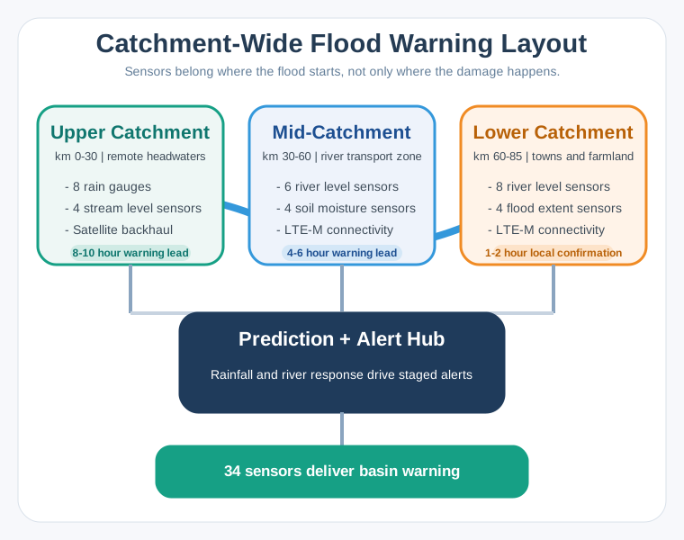
Read from headwaters to valley floor: upstream rain precedes flooding by 6–10 hours. Along the 85 km river, Upper Catchment has eight rain gauges and four stream-level sensors. Its 12 sensors use satellite where cellular coverage is absent and provide 8–10 hours of warning. Mid-Catchment has six river-level and four soil-moisture sensors. These use LTE-M and provide 4–6 hours of warning. Lower Catchment has eight river-level and four flood-extent sensors. These use LTE-M for 1–2 hours of local confirmation. All zones feed the Prediction + Alert Hub for hydrological modelling, edge computing and alerts. The total is 12 + 10 + 12 = 34 sensors. Upstream rain gauges provide advance warning; downstream sensors confirm predictions.
The upper catchment uses satellite because cellular coverage is absent. That choice supplies a working communications path; it does not make the weather measurement more accurate. LTE-M serves the reachable mid- and lower zones.
At the conservative $1.1 million annual avoided-damage estimate, subtract $40,000 annual operations to obtain $1.06 million net annual benefit. The $350,000 capital budget divided by $1.06 million is about 0.33 year, or four months. This annualized quotient does not establish when a particular flood occurs or when savings are realized. Verify that the full support budget and warning response are in place before relying on the modeled payback.
Summary
A rollout case must connect spending to coverage, calibration, adoption, and action. The traffic example requires evidence outside the pilot boundary and a realistic benefit ramp. Beijing’s hybrid plan separates low-cost spatial coverage from reference calibration, while its health benefit depends on routing and alert uptake. The smaller city’s budget shows why a cheaper sensor count still needs a spatial-coverage review.
Flood warning ties placement directly to response time. Upstream observations create the warning window; downstream observations confirm conditions. Compare capital and operating costs over matching horizons, and test the assumptions behind a short simple-payback claim before scaling.
Approve the next rollout stage when evidence connects the installed network to the expected benefit: reliable measurements, actual use, and enough time to act.