27 IoT Deployment Economics: Budget Models
More
Depth: Practitioner
Progress saves as you read. Mark sections complete as you go; your progress appears in the sidebar.
- Podcast audio coming soon
- Character narration audio coming soon
27.1 Build a Budget That Survives Deployment
A traffic sensor pilot can look cheap until installation and support reach every junction. In this chapter, Los Angeles is considering sensors and adaptive timing at 4,500 traffic signals. The proposal promises shorter commutes, but the budget must explain how the whole service becomes operational and what it costs to keep it working. Counting detectors alone cannot answer that question.
We will turn that proposal into a reviewable cost model: separate upfront deployment from recurring operations and replacement, connect benefits to decisions, and calculate payback only after subtracting annual operating costs. This is part 1 of 2; the rollout and ROI evidence chapter then tests how deployment timing changes the claim. Smart-grid, air-quality, flood-warning, and farm-weather comparisons help expose assumptions that a traffic-only spreadsheet might hide.
The method needs basic arithmetic and the ability to interpret cost-benefit tables. If the device-to-decision chain is unfamiliar, start with the IoT Introduction. Comparing phone plans already uses the same basic skill: weigh the initial purchase against continuing charges and the service you actually receive. Here, the additional challenge is that calibration, maintenance, and adoption determine whether the service delivers its promised benefit.
Capital expenditure (CapEx) is the one-time deployment investment, such as hardware, installation, software licences, and integration. Operating expenditure (OpEx) is the recurring cost of connectivity, cloud services, maintenance, and staff. Replacement costs cover device end-of-life cycling. A five-year total cost of ownership (TCO) model brings these costs into one comparison. Return on investment (ROI) relates the benefit to the investment; simple payback asks how long positive net annual benefit takes to recover CapEx.
The problem is to build those rows without claiming benefits before the system can support a useful action. We will first set the operating boundary, then record the assumptions, test data quality, and apply the framework to the traffic budget. Along the way, we will balance cost, coverage, accuracy, and maintainability, quantify benefits with realistic adoption discounts, and examine why calibrated sensor tiers can outperform a uniform network.
KEY CONCEPTS
- Deployment investment
Count hardware, installation, licences and integration.
- Operating cost
Carry connectivity, cloud, maintenance and staff through the lifecycle.
- Trustworthy coverage
Use reference checks to make lower-cost coverage useful.
- Benefit and payback
Adjust benefit for adoption and subtract OpEx before dividing CapEx.
27.2 Part Objectives
- Build capital and operating cost models for an IoT rollout.
- Calculate payback for a smart traffic deployment.
27.3 Scan the Operating Boundary Before the Spreadsheet
The IoT Application Domains examples show how sensing changes across industries. The slide evidence puts very different products beside one another. That contrast is useful before any cost model is built because each example moves the system boundary in a different way:
| Source example | What the slide establishes | Boundary to carry into a worked estimate |
|---|---|---|
| Ant-sized radio | The radio gathers power from the same electromagnetic waves that carry its received signal, so it needs no battery. | Treat available communication energy, not battery replacement, as the power constraint. |
| Smart building | Air-quality and cleaning sensors share a building context, while Ethernet carries power in one direction and data in the other for LED lighting and monitoring. | Include cabling and powered network infrastructure with the sensing plan. |
| Autonomous campus bus | The stated goals are travel-time efficiency, energy saving, reduced road toll, mobility for older people, and lower emissions. | Keep those outcomes separate so one attractive claim does not stand in for all five. |
| Sydney Harbour Bridge | The example places 3,200 vibration sensors under the bridge, uses fibre connectivity, and supports predictive maintenance. | Model installation access, backhaul, and the maintenance decision together rather than pricing sensors alone. |
| Connected dairy farm | Automatic cow identity supports milk-production tracking, while motion supports health monitoring. | Preserve identity and measurement purpose as separate data fields; a tracked animal is not yet a health conclusion. |
These are not interchangeable “smart object” stories. The first is bounded by harvested power, the second by shared wired infrastructure, the third by several public outcomes, the fourth by inspection-scale deployment, and the fifth by the link between identity and observation. A credible worked example starts with that boundary, then adds costs and benefits.
27.4 Turn the Decision into Reviewable Rows
The examples in this chapter are useful because they show the structure of an IoT business case. The exact numbers will change by city, vendor, country, installation labor, connectivity plan, maintenance contract, and sensor quality. The transferable skill is knowing which numbers must be gathered before anyone trusts the result. A calculation is not credible because it has many digits; it is credible when the units, assumptions, owners, and uncertainty are visible.
A good IoT calculation starts with the outcome, then works backward to the sensing system. Traffic timing, air-quality monitoring, flood warning, and farm weather networks all need different hardware, but they share the same accounting pattern: upfront deployment cost, recurring operating cost, replacement cost, measurable benefit, uncertainty, and deployment ramp-up. The first question is therefore not “which sensor is cheapest?” It is “which decision will improve, how often does that decision happen, and how much better must the system make it to justify the operating burden?”
The IoT Common Pitfalls chapter examines mistakes to avoid. Here, the accounting pattern prevents two common mistakes. One mistake is treating the bill of materials as the whole project, leaving out mounting, power, permissions, site visits, calibration, spares, cloud storage, dashboards, integration, cybersecurity review, and support. The other is treating annual benefits as if they appear on day one, even though real deployments phase through procurement, permits, installation, commissioning, user training, and slow adoption. The worked examples make those hidden assumptions visible before they turn into a budget surprise.
- Cost side: Devices, sensors, gateways, mounting, enclosure, calibration, connectivity, cloud, integration, support, and replacement.
- Benefit side: Time saved, damage avoided, energy reduced, compliance improved, uptime gained, or decisions made earlier.
- Uncertainty side: Adoption rate, weather variability, failure rate, maintenance access, data quality, and delayed rollout.
Use the scenarios as calculation templates, not as current price lists. Copy the structure, then replace the assumptions with locally sourced evidence: quotes from vendors, installation estimates from contractors, historical incident records, maintenance logs, cellular or LoRaWAN coverage checks, cloud retention policies, and the decision threshold that determines whether the data is good enough to act.
A shared accounting pattern becomes useful when each row can be challenged and updated.
When building a real project estimate, do not hide assumptions inside a headline ROI. Put each assumption in a row with an owner and a source. A LoRaWAN flood gauge, LTE-M air-quality node, Wi-Fi traffic controller, or BLE environmental logger will have different radio coverage, power, enclosure, calibration, and support costs. If a row says “sensor cost,” split it into device, sensor element, enclosure, mast or mount, power supply, antenna, SIM or network join process, commissioning labor, spares, and replacement interval.
The IoT Business Models chapter develops monetization and pricing strategies; this worksheet must still identify whose benefit each row represents. The same rule applies to benefits. A traffic example may price driver time. An air-quality example may depend on health-risk models and policy adoption. A flood-warning example may use expected annual damage. A farm-weather example may depend on frost events and grower behavior. Each one needs a sensitivity check before the payback claim is credible. A single ROI value is less useful than a small table showing conservative, expected, and optimistic cases for deployment speed, adoption, avoided loss, maintenance cost, and sensor failure.
- Define the unit. State whether the cost is per sensor, intersection, gateway, field, building, or year.
- Separate one-time and recurring costs. Keep CapEx, OpEx, replacement, and staffing in different rows.
- Run conservative and optimistic cases. Vary adoption, sensor failure, maintenance visits, connectivity cost, and deployment time.
For a field-ready worksheet, add columns for assumption, unit, quantity, unit cost, timing, source, owner, confidence, and sensitivity range. The source column matters. A vendor quote, a procurement catalog, a city incident database, a maintenance log, and an engineer’s estimate deserve different confidence. The owner column matters too, because someone must be able to update the row when the radio plan changes, labor rates change, or a pilot shows that the maintenance interval is wrong.
Finally, link each cost to a decision. If an air-quality node does not change where warnings are issued, where enforcement happens, or how exposure is reduced, its benefit row is weak. If a flood gauge does not change warning lead time, evacuation action, or asset protection, its benefit row is weak. If a farm-weather station does not change irrigation, frost response, or disease-risk decisions, its benefit row is weak. The spreadsheet should make this trace from sensor to action explicit.
27.5 Make Data Quality Part of the Cost Model
Cheap sensors create coverage, but coverage is useful only when the data can support the decision. A PM2.5 network may combine reference stations, mid-grade optical sensors, and low-cost nodes because calibration drift, humidity, placement, and cleaning affect the measurement. A flood-warning network may prioritize upstream stage gauges, rain gauges, telemetry reliability, and battery-backed gateways over uniform spacing. A traffic network may spend more on controller integration, cabinet access, failsafe timing plans, and fiber or cellular backhaul than on the detector itself.
The technical design must therefore connect cost to data quality. MQTT, CoAP, HTTP APIs, or vendor cloud connectors can move readings, but the business case also needs timestamps, units, calibration state, quality flags, missing-data rules, and maintenance records. Without those, the spreadsheet may look precise while the field system cannot support the decision it promises. For example, a cheap air-quality node without humidity correction and reference calibration may be inexpensive per device but expensive per trustworthy decision.
The complete cost path in Figure 1 connects data quality to the business case. CapEx, OpEx, realised benefits, adoption, and investment metrics must all use the same deployment and operating assumptions; otherwise a cheap sensor can look economical while producing expensive or unusable evidence.
- Calibration: Budget for reference checks, drift correction, sensor cleaning, and replacement intervals.
- Availability: Include radio coverage, gateway redundancy, local buffering, battery reserve, and repair access.
- Decision quality: Define the minimum spatial density, latency, accuracy, and confidence needed for the action.
The financial model should include the same state transitions that the system must manage: ordered, installed, commissioned, online, calibrated, degraded, offline, repaired, and replaced. Benefits should ramp with those states, not with an idealized launch date. A sensor that is installed but uncalibrated should not count as full data coverage. A gateway that buffers locally during an outage should have different data-loss risk than a device that drops readings. A dashboard that reports stale values should be treated differently from one that marks missing data explicitly.
This is why tiered designs often beat uniform designs. Reference stations, anchor gauges, or high-confidence locations may cost more, but they make the cheaper layer useful by providing calibration, validation, and decision thresholds. The economic question is not the average sensor price; it is the cost per reliable action over the life of the deployment.
In these examples, a small high-accuracy layer of 5–10% supports calibration of broad lower-cost coverage of 90–95%. Those proportions describe a tiered plan, not a universal placement rule. Choose sensor numbers, density, and locations from the measurement, maintenance, and warning requirements. A larger node count improves spatial coverage only where that extra coverage improves the decision.
The Concept Navigator can help connect calibration, availability, and decision quality when a budget assumption needs further explanation.
27.6 Test the Pattern on a Small Budget
Before scaling to 4,500 intersections, use Temperature Terry’s farm frost example to check the accounting. Saving allowance for a purchase explains the first bill; the project must also pay its running bills every year. Terry needs 30 temperature-sensing units, each with power and a radio.
| Item | Calculation | Upfront cost |
|---|---|---|
| Temperature sensors | $10 × 30 | $300 |
| Solar panels | $25 × 30 | $750 |
| Wi-Fi radios | $15 × 30 | $450 |
| Total CapEx | $1,500 |
Internet service costs $5/month, or $60/year. Replacing broken sensors adds $100/year, making annual running costs $160. Buying equipment is CapEx; running the service is OpEx. Keep the replacement allowance visible even when it is grouped into the annual operating budget, so it is not counted again elsewhere.
Assume frost damages $2,000 of crops each year and the system prevents 80% of that damage. Avoided loss is $2,000 × 80% = $1,600/year. Subtracting the $160 running cost leaves $1,440/year in net savings. Simple payback is $1,500 / $1,440 = about 1 year. These assumptions show how sensors can save more than they cost, while making clear that the savings depend on avoided damage and continuing operation. After payback, net savings continue only while those assumptions hold; operating and replacement costs do not disappear.
Always add up the whole system, rather than just the temperature sensor. The same discipline will expose why a city-wide traffic upgrade costs far more than a detector purchase, and why a large claimed saving still needs an adoption and rollout check.
27.7 IoT Cost-Benefit Framework
Terry’s small budget and the city’s traffic proposal use the same framework. Keep deployment investment, annual operating cost, and benefits separate until each has a stated basis.
Figure 1 sets out the order of work that every example in this chapter follows.
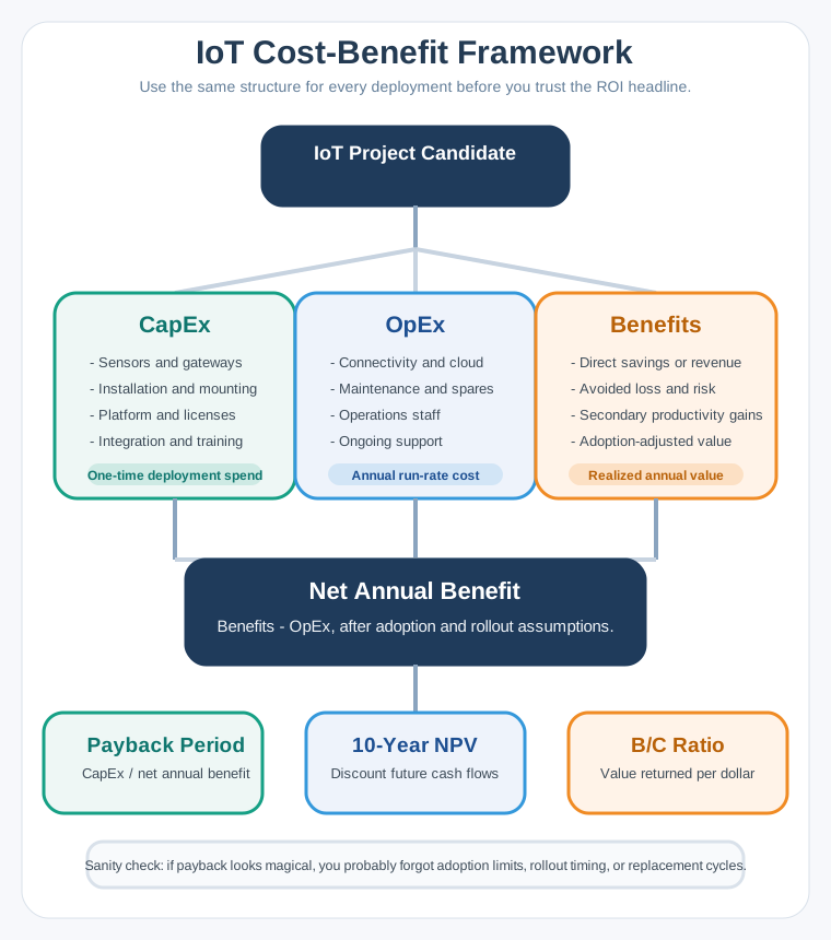
The candidate project at the top of Figure 1 splits three ways, and keeping those branches apart is the whole discipline. CapEx is one-time: hardware, mounting, licences, and the integration work that is usually underestimated. OpEx is the yearly run rate that never stops, from connectivity to the staff who watch the dashboards. The benefits branch is deliberately adjusted for adoption, because a saving nobody takes up is not a saving. Subtract annual OpEx from adoption-adjusted annual benefit to obtain net annual benefit. Use it with CapEx for payback; ten-year net present value (NPV) also needs discounting and timing, while benefit-cost ratio compares benefits with costs. The warning at the foot is worth keeping: if a payback looks magical, check adoption, rollout, and replacement first.
The five worked examples across the budget and coverage routes apply this framework to progressively different domains. Each example highlights a different scale and design pattern:
- Smart traffic: Urban mobility at 4,500 intersections; city-wide deployment matters more than isolated pilots.
- Beijing air quality: Megacity health monitoring with 29,911 sensors; hybrid reference and low-cost sensors make block-level coverage affordable.
- Generic air quality: A mid-size city network with about 95 stations; three sensor tiers balance regulatory accuracy with spatial coverage.
- Flood warning: Agricultural safety across 34 sensors; catchment-wide distributed sensing creates useful lead time.
- Weather network: Precision agriculture with 51 stations and loggers; terrain-aware placement beats uniform grids.
With the pattern in place, the first example deliberately starts at large scale. Traffic exposes the danger of reading a huge ROI number without asking when the system actually becomes operational.
The companion Coverage and Decision Tools route develops coverage choices beyond this first budget. The framework also lets you compare smart-grid and environmental proposals without assuming they have identical benefit mechanisms.
The figures are scenario data for learning the calculation method. Costs vary by region, vendor, labor market, procurement model, connectivity plan, sensor quality, maintenance contract, and scale. Use the examples as calibration prompts, not fixed values or current market quotes. The methodology is the transferable skill.
27.8 Smart Traffic Signal Optimization Budget
Now apply the same rows to the running scenario: Los Angeles, California (population 3,970,000) plans to upgrade 4,500 traffic signals with IoT sensors and adaptive timing to reduce average commute times by 12%.
Given:
- Current traffic signals: 4,500 across 503 square miles
- Assumed one-way commute: 32.5 minutes; no current national ranking is assumed.
- Daily commuters: 1.85 million people
- Signal upgrade cost: $18,500/intersection (sensors, controller, connectivity)
- Adaptive timing software: $2.4M platform license + $890K/year
- Emergency vehicle preemption: Additional $4,200/intersection
- Assumed driver hourly value: $28.50 (attributed to the BLS median wage in the source example; no date supplied)
Steps:
-
Calculate current commute cost:
- Daily commute hours: 1.85M commuters x (32.5 min x 2) / 60 = approximately 2.0M hours/day
- Annual commute hours: 2.0M x 250 workdays = approximately 500M hours/year
- Annual commute cost: 500M x $28.50 = $14.25 billion/year
-
Calculate deployment costs:
- Signal upgrades: 4,500 x $18,500 = $83.25M
- Emergency preemption: 4,500 x $4,200 = $18.9M
- Platform software: $2.4M
- Installation labor: $12.5M (estimated)
- Total CapEx: $117.05M
-
Calculate annual operating costs:
- Software license: $890,000/year
- Connectivity: 4,500 signals x $35/month = $1.89M/year
- Maintenance (8% of hardware): $8.2M/year
- Operations team (15 FTE): $2.1M/year
- Total OpEx: $13.08M/year
-
Calculate time savings at 12% reduction:
- Commute reduction: 32.5 min x 12% = 3.9 minutes saved per trip
- Annual hours saved: 500M x 12% = 60M hours/year
- Dollar value: 60M x $28.50 = $1.71 billion/year
-
Calculate secondary benefits:
- Fuel savings (15% idle reduction): $340M/year
- Emissions reduction: 180,000 tons CO2/year
- Accident reduction (8% fewer intersection crashes): $125M/year in damages
- Assume emergency preemption shortens response by 2.1 minutes; 45 lives per year remains an unvalidated outcome hypothesis, excluded from the calculated benefit.
- Secondary benefits: $465M/year
-
Calculate ROI:
- Total annual benefit: $1.71B + $0.465B = $2.175B
- Net annual benefit: $2.175B - $13.08M = $2.162B
- Simple payback: $117.05M / $2.16192B = 0.05414 years, or about 19.8 days at 365 days/year
- 10-year NPV (5% discount): approximately $16.58 billion, assuming ten equal year-end net benefits and upfront CapEx.
Result: Using the rounded 500M annual commute hours, the $117.05M investment has about $2.162B in net annual benefit and a steady-state simple payback under 3 weeks. The original shorthand is a $117M investment and $2.16B annual net benefit. Each $1 invested corresponds to $18.47 in annual net benefit under these assumptions. This includes the dollar value of commuter time; it should not be read as $2.16B of cash available to the city’s budget. The 12% commute reduction is an example input; Carnegie Mellon’s Pittsburgh Surtrac deployment reported a 25% reduction in average travel times. Carnegie Mellon
The large result comes from applying a time saving to millions of commuters every day. It demonstrates the sensitivity of the method, rather than establishing that traffic optimization has the highest ROI of every smart-city investment. Successful timing changes require coordinated coverage: isolated smart intersections can create traffic waves at adjacent traditional signals. Budget phased coverage and measure the effects at adjacent signals before extending the benefit claim city-wide.
Rounding also matters. The commute inputs give 2.00417M hours/day and 501.04167M hours/year before rounding, rather than exactly 2.0M and 500M. The worked budget deliberately carries the rounded 500M baseline into its $14.25B commute cost, 60M hours saved, and $1.71B time benefit. Keep that convention visible instead of mixing rounded and unrounded branches. Maintenance is likewise an approximately $8.2M allowance, and all payback and NPV results depend on the stated operating costs.
The estimate assumes full recurring benefits. It does not yet establish when procurement, installation, commissioning, and adoption produce them. That distinction is the reason to carry this budget into the rollout chapter rather than treating a steady-state payback as elapsed time from approval.
For other interactive calculation tools, use the Simulation Playground after recording the assumptions that the tool should vary.
Summary
A reviewable IoT budget starts with the decision and its operating boundary. It separates CapEx, OpEx, and replacement across a five-year ownership comparison, then connects every benefit to an action that the deployed service can support. Record units, sources, owners, timing, and uncertainty so the estimate can change when field evidence changes.
Calibration, availability, and placement determine whether coverage is useful. Tiered sensing can extend coverage economically when reference checks keep measurements trustworthy. In the traffic example, the large time benefit makes simple payback look short, but it remains conditional on coordinated deployment, adoption, and continuing operations. A precise spreadsheet cannot replace that evidence.
Budget the cost per reliable action over the deployment’s life. Subtract recurring costs from realised benefits, then test when those benefits can actually begin.
Carry the budget into IoT Deployment Economics: Rollout and ROI Evidence, beginning with the partial deployment trap.