17 IoT Systems Evolution: Computing and Placement
More
Depth: Practitioner
Progress saves as you read. Mark sections complete as you go; your progress appears in the sidebar.
- Podcast audio coming soon
- Character narration audio coming soon
17.1 Decide Where the Sensor System Thinks
Computing improved, but a sensor system still cannot send every byte to an unlimited cloud without cost, delay, or energy consequences. This chapter connects computing economics to the practical question of where processing belongs. You will explain distributed-computing economics, choose device, edge, fog and cloud placement from requirements, and test evolution claims against power and architecture evidence.
Keep the factory team in view: its sensors feed decisions that must eventually reach actuators. Some work needs immediate local response; other work benefits from site coordination or long-term fleet history. The team must explain why distributed placement helps a particular workload before claiming it saves money. Later, the farm case tests the same reasoning against slower irrigation decisions and uneven coverage.
This is part 2 of 2. Review IoT Systems Evolution: Cycles and Convergence for the first route. The problem here is to separate useful hardware progress from a complete-system decision. We will first examine the economics, then compare placement approaches against latency, bandwidth, power, privacy and resilience.
KEY CONCEPTS
- Efficient computing
More capability per chip widens placement options.
- Workload placement
Put urgent action near the physical process.
- Energy budget
Sleep, sensing and radio use determine field life.
- Complete-system cost
Count the node, network and ongoing service.
17.2 Learning Objectives
By the end of this chapter, you will be able to:
- explain the economics of distributed IoT computing
- choose edge, fog, and cloud placement from requirements
- test evolution claims against power and architecture evidence
17.3 Follow the Economics Beyond Clock Speed
Earlier economics often favoured centralised compute
When single-core performance was still improving rapidly (30–40% per year), faster central servers made economic sense for data processing. Devices could remain simple sensors sending data, while data centres supplied the fastest CPUs.
Later economics widened compute-placement options
When single-core performance growth slowed, chip manufacturers emphasised multi-core processors with 2, 4, 8, 16+ cores per chip, specialised accelerators such as GPUs for graphics and NPUs for AI, and performance per watt rather than raw speed alone.
The change becomes concrete in microcontrollers, the processors built into sensor nodes. These historical product examples show different combinations of price and capability; they are not equivalent benchmark results.
| Microcontroller | Year | Price | Capabilities |
|---|---|---|---|
| Intel 8051 | 1980 | $5-10 | 8-bit, 12 MHz, no networking |
| ARM Cortex-M0 | 2009 | $0.50-1 | 32-bit, 48 MHz, low power |
| ESP32 | 2016 | $2-4 | Dual-core 240 MHz, Wi-Fi/Bluetooth, 520KB RAM |
| Raspberry Pi Pico | 2021 | $4 | Dual-core 133 MHz, 264KB RAM, extensive I/O |
A $0.50 microcontroller and a $10,000 desktop computer from 1995 serve different workloads. Price and clock rate alone do not establish which has more useful computing power; compare memory, I/O, application performance and energy.
Local inference and sensor fusion
The proliferation of specialized neural network accelerators makes on-device AI feasible:
- Google Coral Edge TPU: 4 trillion operations/sec, $25, 2W power
- NVIDIA Jetson Nano: 472 GFLOPS, $99, 5-10W power
- Apple Neural Engine: 15.8 trillion ops/sec, integrated in phones
On-device camera inference can reduce upstream video traffic substantially; quantify bandwidth reduction for a defined resolution, frame rate and upload policy.
Modern IoT devices can fuse data from multiple sensors in real-time:
- Smartphones: 24+ sensors (accelerometer, gyroscope, magnetometer, GPS, barometer, light, proximity, etc.)
- Drones: inertial measurement unit (IMU) (9-axis), GPS, ultrasonic, optical flow, cameras - all fused for stable flight
- Wearables: Heart rate, ECG, SpO2, temperature, accelerometer combined for health insights
Give each layer a job
A fog architecture coordinates processing across intermediate nodes between devices and cloud services. This hierarchy gives each layer a distinct job:
- Device layer: Immediate response (sensor -> actuator in <10 ms)
- Edge layer: Local analytics (factory floor aggregation)
- Fog layer: Regional processing (city-wide traffic optimization)
- Cloud layer: Long-term storage and complex AI training
Inspect Figure 1 to decide which work belongs near the physical process and which benefits from wider coordination.
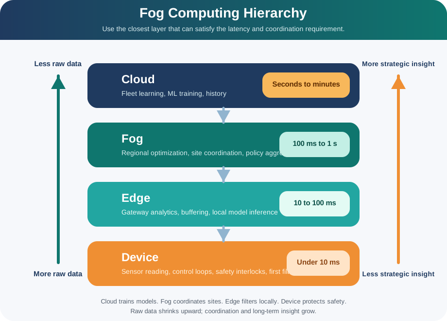
Read Figure 1 upward from immediate sensor-to-actuator work below 10 ms. Edge systems perform local analysis, fog nodes coordinate a site or region, and cloud platforms keep long histories or train complex models. Raw data should shrink as it moves upward while the value and scope of insight increase. In the example, a temperature sensor produces 10 readings each second; the edge reports a trend, and the cloud compares trends across thousands of assets to predict failures. Placement follows response time, bandwidth, privacy, resilience, and coordination needs rather than a fixed edge-first rule.
Ideal Dennard scaling linked smaller dimensions with lower voltage and roughly controlled power density. Real technologies increasingly departed from that ideal: across the early-to-mid-2000s, leakage, power density, interconnect and thermal constraints slowed reliance on frequency growth alone. Multicore, efficiency and specialised logic combined with integration and falling MCU and radio costs to widen endpoint options.
17.4 Test the Claim Before Buying the Architecture
Those capabilities create choices, but they do not settle the factory’s design. Four common claims obscure the difference between a connected endpoint and a useful system.
Misconception 1: “IoT is just about connecting things to the internet.” Simple connected sensors are valid IoT endpoints. Local intelligence is an architecture choice used when latency, resilience, privacy, bandwidth or safety justifies processing near the physical process.
Misconception 2: “Moore’s Law ended, so computing improvement stopped.” Long-run transistor-density gains continued after real technologies departed from ideal Dennard scaling. Benefits increasingly appeared through multicore designs, specialised accelerators, integration and energy efficiency rather than frequency growth alone.
Misconception 3: “Cloud computing and IoT are competing approaches.” Cloud and edge are complementary, not competing. Modern IoT architectures use both: edge devices handle time-sensitive sensing and local actuation, while cloud services handle long-term storage, model training and fleet coordination. The mid-2000s power-efficiency pivot was one contributor to wider placement options; integration, component costs, networks, software platforms and application demand also mattered.
Misconception 4: “IoT just needed cheaper hardware to happen.” Lower component cost was one contributor, not a prerequisite acting alone. Practical deployments also depended on suitable sensors and radios, network coverage, protocols, software platforms, device management, security, integration effort and application demand.
The same distinction matters when the team turns a technology claim into a budget. Check the following failure modes before selecting a design.
Pitfall 1: Assuming “newer era = abandon previous era” Each computing era builds on top of previous ones rather than replacing them. Companies that rip out centralized servers in favor of edge-only architectures discover they still need cloud for ML training, fleet management, and long-term analytics. The correct approach is a complementary multi-tier architecture, not wholesale replacement.
Pitfall 2: Extrapolating Moore’s Law linearly into device cost A $0.50 microcontroller does not mean a $0.50 IoT device. The bill of materials (BOM) for a complete IoT node includes the MCU ($0.50-$4), wireless radio ($1-$5), antenna ($0.20-$2), power regulation ($0.50-$2), sensors ($0.50-$10), PCB and assembly ($1-$5), and enclosure ($1-$10). Estimate complete-node BOM from MCU, radio, sensor, board, enclosure, assembly and test for the production volume. Budget accordingly.
Pitfall 3: Ignoring the “last mile” of the 10x cycle The active-IoT-device trajectory is in tens of billions, not a documented “next trillion”; IoT Analytics forecast 39 billion by 2030. Some proposed last-mile deployments target sub-$1 hardware, 10+ year battery life, and operation in harsh environments (underwater, underground, extreme temperatures). Do not assume the next 10x will arrive at the same pace as previous cycles — physics and economics impose harder constraints at each step.
Pitfall 4: Confusing clock speed with real-world performance Compare application workload, memory, radio and power budget rather than clock rate alone. Modern microcontrollers have hardware peripherals (DMA, hardware crypto, radio baseband) that offload work from the CPU. For sensor reading, protocol handling and local inference, compare the $4 MCU with the $500 desktop on the actual workload. Hardware offload can help with I/O-bound work; it does not establish a general performance ranking.
The illustrative 2005–2025 cost comparison illustrates the intended direction of change: microcontrollers at $5–10 versus $0.50–2, wireless modules at $50–100 versus $2–5, cloud storage at $1 versus $0.01 per GB-month, and sensors at $10–50 versus $0.20–2. Its MCU power examples are about 100 mW typical versus 50 mW active and 5 mW asleep; its example complete-device total falls from about $200+ to $5–20. These are illustrative entries, not dated, comparable product benchmarks. Active and sleep power are different operating states, so they cannot support one improvement ratio. A defensible cost or efficiency trend needs named products or tariffs, dated specifications and a common workload.
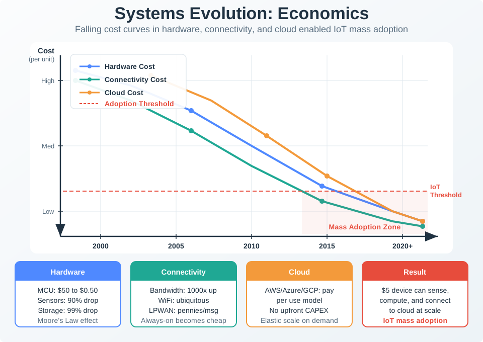
Read the 2005 and 2025 columns from microcontroller cost and power through wireless modules, cloud storage, and sensors. Then compare the total device costs, from about $200+ to about $5–20. The power row compares typical, sleep, and active states, so it gives no single efficiency ratio. Lower entry costs can make more deployments viable, but costs across the system’s life still matter. Network and cloud use also carry running costs. A claim of 100× better performance per watt needs a dated test of the relevant device class. The factory should get quotes for complete nodes and measure energy use before buying. These historical examples cannot replace its own budget.
17.5 Audit the Factory’s Upfront and Annual Costs
With the limits of the historical comparison clear, return to the factory. The following alternatives isolate compute and bandwidth costs; they do not yet price equivalent complete systems.
Real-World Example: Smart Factory Comparison
Illustrative centralized baseline:
- 1,000 sensors -> Central server processes all data -> Actuators respond
- Latency: 100-500 ms (sensor -> cloud -> actuator)
- Bandwidth: 1 Gbps fiber needed for real-time data
- Single point of failure: Server down = factory stops
- Cost: $100K server + $50K/year bandwidth
Illustrative distributed alternative:
- 1,000 smart sensors with $2 microcontrollers -> Local edge processing -> Immediate actuation
- Latency: 1-10 ms (sensor -> edge -> actuator)
- Bandwidth: 10 Mbps (only aggregate data to cloud)
- Resilient: Local loops continue if cloud fails
- Cost: $2K in microcontrollers + $1K/year bandwidth
Savings: $98K upfront + $49K/year by distributing computing to edge devices
The $98K difference is $100K minus $2K in selected compute hardware; the $49K annual difference is $50K minus $1K in bandwidth. Before accepting either as a deployment saving, include complete BOM, gateways, networks, software, installation, operations and failure impact on both sides. Measure end-to-end latency and traffic for the same required functionality. Local loops can continue through a cloud failure only when the local design provides that autonomy.
17.6 Connect the Enablers to Useful Patterns
The factory’s alternatives became practical through several changes working together. None alone explains the timing or the best placement.
1. Abundant Cheap Computing
- Moore’s Law describes a long-run transistor-density trend, not a guaranteed doubling schedule or complete-device cost forecast
- Focus shifted from speed to efficiency and specialization
- $0.50 microcontrollers put useful local computation within reach; compare workloads before equating them with 1990s desktops
2. Energy Efficiency Revolution
Energy claims require a defined workload and operating state.
- Battery-powered devices can run for years
- Energy harvesting becomes viable for some applications
3. Specialized Accelerators
- Neural network accelerators: AI on $25 chips
- Cryptographic engines: Secure communication with minimal overhead
- Radio modules: Wi-Fi/Bluetooth/LoRa on single chip
Result: Continued integration, lower-cost components, improved efficiency, networking, software platforms and application demand jointly widened the range of practical connected products.
Why scale arrived gradually
Several trends converged over time:
- Earlier deployments: Distributed nodes often faced higher component, power, integration and operating costs, so central processing remained attractive for many workloads.
- Mid-2000s onward: Power and thermal constraints increased emphasis on efficiency, multicore processors and specialised logic.
- 2010s: Continued integration, lower-cost MCUs, radios and sensors, broader networking, cloud and device platforms, and maturing protocols reduced deployment friction.
- Later deployments: Edge accelerators and improved tooling widened the workloads that could run near physical processes.
The mid-2000s power-efficiency pivot was one contributor. Continued integration, lower-cost microcontrollers, radios and sensors, networking, software platforms and application demand jointly widened practical IoT and edge-computing options.
Choose the pattern from its job
These converging technology and deployment trends support the architectural patterns studied later in this module:
- Edge Computing: Places work near devices when latency, resilience, privacy or bandwidth justifies it
- Fog Computing: Hierarchical processing uses intermediate nodes whose capabilities depend on the workload
- Edge AI/ML: Can use specialized neural accelerators available in $25 chips
- Wireless Sensor Networks: Nodes need computation for routing, data fusion, and coordination
No single event produced these patterns. Hardware integration and efficiency, component cost, networks, software platforms and application demand converged to widen useful compute-placement choices.
Figure 3 shows the four patterns as peers fed by one shared set of causes.
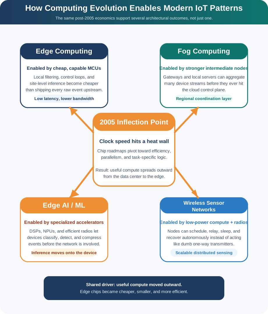
Start in the panel on the left, which lists the joint contributors: cheaper microcontrollers, radios and sensors, better networks, software platforms, and demand from applications. The four arrows leaving it carry the same label, and that repetition is the claim, because no single advance produced any one pattern. Now read across the four cards. Each names the capability it leans on and the work it actually does, so edge AI is tied to accelerators and local inference, while sensor networks are tied to computation at the node for routing and fusion. The line at the foot of Figure 3 is the one to carry forward: choose placement by constraint, not by slogan.
Device Evolution follows the Embedded → Connected → IoT progression, while IoT History examines lessons from those transitions. Industrial IoT Fundamentals places the factory’s computing choices in the Fourth Industrial Revolution context.
The five phases of connectivity run from connecting computers (1969), through connecting people (1991–2012), to connecting things (2010+). Each builds on earlier infrastructure. Treat the “10× cycle” as a teaching heuristic, not a measured law of 1,000× more devices or 1/100th cost. The 39 billion active-connection forecast for 2030 is a forecast, not evidence for an inevitable next trillion.
17.7 Place Work Against the Actual Constraints
Hardware integration and efficiency, lower component costs, networking and software platforms widened edge-processing options, but placement remains a workload decision. Use this framework to decide where intelligence belongs.
Use these placement questions as a compact decision matrix:
- Latency requirement: process at the edge when the action must complete in under 100 ms; cloud is reasonable when a network round trip of roughly 50-200 ms is acceptable.
- Data volume: process high-volume streams, such as video, near the source; send compact events or summaries to cloud services.
- Connectivity reliability: keep safety and continuity logic local when links are intermittent; use cloud processing when the connection is reliable.
- Power budget: let sleepy edge devices duty-cycle when the radio is expensive; use cloud processing when the device can afford continuous communication.
- Processing complexity: run simple inference and rules locally; reserve training, multi-model analysis, and heavy storage for cloud services.
- Security and privacy: keep sensitive biometric, health, or operational data local where possible; transmit only the derived evidence the workflow needs.
- Fleet learning: use cloud aggregation when cross-site learning matters; keep isolated fast-response logic at the edge.
- Device cost: choose edge AI only when the product can afford the $10-$50 compute path; use a cheaper MCU plus radio when thin-edge telemetry is enough.
Four ways to assign the work
Apply those questions to four examples. Their figures are scenario assumptions, not universal performance or pricing guarantees.
Edge-only suits the illustrative industrial safety system that cuts power to machinery when it detects a hazard. Its 10 ms requirement and need to work during network outages put the decision locally. A $25 microcontroller runs a local ML model; this fully autonomous example has no cloud role.
Cloud-only, with a thin edge, suits the battery-powered parking sensor reporting binary occupied/vacant state every 30 seconds. The example has no urgent actuation deadline. A $2 MCU and LoRaWAN radio send the observations; cloud services perform occupancy analysis, pricing optimisation and reporting.
Hybrid edge inference and cloud training divides the security camera’s work. A $35 processor with a neural accelerator detects faces at 30 fps, keeping face processing local. The illustrative 99% bandwidth reduction against raw-video streaming must be checked against resolution, frame rate and upload policy. Cloud services train updated face-detection models weekly using edge-collected metadata rather than faces.
Tiered device, gateway and cloud processing groups a factory’s 500 sensors behind 5 edge gateways. Each $200 gateway, specified here with a 16-core processor, aggregates and filters data from 100 low-cost sensors at $2 each. The gateways handle real-time aggregation; cloud services provide long-term storage, cross-factory optimisation and predictive fleet models.
17.8 Work Through the Farm’s Trade-offs
The factory’s urgent actuation favours local response. The farm scenario asks a different question: how much local processing does irrigation need when most measurements can wait?
Scenario: 500-acre farm needs soil moisture monitoring to optimize irrigation.
Option A: Cloud Processing
- Sensor: $12 (MCU + LoRaWAN radio + moisture probe)
- Sends reading every 15 minutes to cloud
- Cloud analyzes all 50 sensors, sends irrigation commands
- Latency: 5-30 seconds
- Cost per sensor: $12 hardware + $3/year connectivity = $15 in the first year
- 50-sensor network: $600 hardware + $150/year OpEx = $750 in the first year
Option B: Edge Gateway Processing
- Sensor: $8 (simple analog probe + LoRaWAN)
- Edge gateway: $350 (solar-powered, runs local irrigation optimization model)
- Gateway reads 50 sensors every 5 minutes, controls irrigation valves locally
- Cloud used only for historical storage and model updates
- Latency: <1 second (local control loop)
- Cost: $400 sensors + $350 gateway + $30/year connectivity = $780 in the first year
Option C: Hybrid Approach
- 45 low-cost sensors ($8 each): Report to cloud every 30 min
- 5 reference sensors ($50 each): Edge processing for critical zones with 1-minute local control
- Cloud analyzes 45-sensor trends, local edge handles fast response in critical areas
- Cost: $360 + $250 = $610 hardware + $75/year OpEx
Decision Factors:
- Irrigation response time: Crops can tolerate 5-30 second delays (cloud OK), except in sandy soil zones (need edge)
- Connectivity: LoRaWAN coverage good but not perfect (edge provides autonomy)
- Learning: Cloud aggregates multi-field patterns for better predictions (cloud advantage)
Optimal Choice: Option C (Hybrid)
- Combines low-cost broad coverage (cloud) with fast local control where needed (edge)
- First-year selected costs are $685 ($610 + $75), about 12.2% below Option B’s $780; the $610 hardware alone is about 18.7% below Option B’s $750 hardware
- Better responsiveness than pure cloud (Option A) for critical zones
The choice follows the scenario’s critical-zone needs, not a rule that every farm requires fast edge control. Compare the stated 15-minute, 5-minute, 30-minute and 1-minute reporting or control intervals with the application’s tolerated delay. Keep hardware expenditure separate from annual operating cost when comparing these alternatives.
17.9 Cost Curves: When Edge Becomes Cheaper
Check the cost curve’s assumptions
The illustrative breakeven cases isolate selected communication and compute costs:
| Data Volume | Breakeven Device Count | Explanation |
|---|---|---|
| 10 kB/sec | 1 device | Even 1 device streaming 10 kB/sec costs $15/month cellular; $50 edge chip takes about 3.3 months to recover at $15/month |
| 1 kB/sec | 10 devices | $1.50/month cellular × 10 = $15/month; edge gateway ($200) pays back in about 13.3 months |
| 100 bytes/sec | 100 devices | LPWAN costs $3/year/device, cloud competitive; edge only if latency matters |
Key insight: Technology convergence widened edge-processing options, but the appropriate architecture depends on latency, data volume, connectivity, power, privacy, safety and fleet-learning constraints. There is no universal “always edge” or “always cloud” answer.
These device counts are scenario entries, not universal thresholds. The 100-bytes/sec case establishes no numerical edge payback from the information given. Add the gateway or device cost, remaining traffic and service costs before treating a row as a business case.
17.10 Quick Decision Algorithm
The quick decision algorithm prioritises edge processing when latency must be below 100 ms, connectivity is unreliable, or data volume exceeds 1 MB/sec. Otherwise, high processing complexity or fleet learning favours cloud; a tight budget with latency tolerance above 5 seconds favours thin-edge telemetry; the remaining case suggests hybrid edge inference and cloud training.
These thresholds are screening questions. They do not prove that edge processing is required or that a cloud path meets a deadline. The main decision matrix also uses a roughly 50–200 ms network round trip as an example of acceptable cloud timing. Measure the chosen path, including sensing and actuation, and retain local safety and continuity logic wherever remote delay or outage would violate the requirement.
Power management belongs in the same decision. A sleepy device can duty-cycle when radio use is expensive. Battery-powered devices can run for years and energy harvesting can suit some applications, but a 10-year field claim requires measured sleep current, wake energy and radio use, together with battery derating, temperature, ageing, self-discharge and reserve margin. Transistor density alone cannot establish that life.
Summary
Computing economics widened the work that sensor nodes can do, while networks, software platforms, integration and application demand made larger deployments practical. The departure from ideal Dennard scaling increased attention to efficiency, multicore designs and specialised logic; it was one contributor among several.
The factory and farm show why complete-system boundaries matter. Separate upfront hardware from recurring service, test latency and bandwidth on the actual workload, and assign immediate action, local analysis, regional coordination and fleet learning to appropriate layers. Edge and cloud remain complementary. More local intelligence earns its place when it meets the application’s constraints and justifies its lifecycle cost.
Choose compute placement from the workload’s response time, data volume, connectivity, power, privacy, safety and learning needs, then verify the complete-system economics.
Carry those decisions into IoT Perspectives, where stakeholder roles change how the system’s value is judged.