24 Accuracy, Precision, Drift, and Hysteresis
24.1 Start With the Measurement Story
A tidy graph can hide three different problems: readings can be wrong, scattered, or slowly moving over time. The first step is to separate accuracy, precision, drift, hysteresis, and repeatability before choosing a fix.
24.2 Learning Objectives
After this page, you should be able to:
- Distinguish accuracy, precision, drift, hysteresis, resolution, and uncertainty.
- Explain why averaging improves random scatter but does not remove systematic bias.
- Use bidirectional tests to expose hysteresis and time-based tests to expose drift.
- Build a practical error budget instead of trusting displayed decimal places.
- Choose the matching remedy: calibration, averaging, bandwidth control, recalibration, characterisation, or uncertainty reporting.
24.3 Why This Follows Common Sensor Mistakes
Common Sensor Mistakes prevents the obvious failures: voltage mismatch, missing pull-ups, bad warm-up timing, invalid readings, overpolling, address conflicts, analog-reference errors, missing decoupling, long wire runs, and environmental blind spots. After those are handled, the next common failure is misclassifying the remaining measurement error.
Use this page when the sensor works but the number still cannot be trusted. A tight cluster in the wrong place needs calibration, not a longer moving average. A value that changes month by month needs drift evidence and recalibration. A pressure or position reading that differs by direction needs hysteresis testing. The first step is naming the error correctly.

Phoebe’s Why
An ADC’s resolution and a sensor’s accuracy are physically unrelated quantities, which is exactly why this page insists on naming the error before choosing a fix. Quantization error comes from rounding a continuous voltage to the nearest of \(2^N\) steps – a uniformly distributed rounding error whose noise floor shrinks by about 6 dB for every extra bit. Sensor accuracy is a bias or gain error against a physical reference, and it does not care how finely the ADC slices its input range. Averaging shrinks random scatter as \(1/\sqrt{N}\), the same math behind this page’s 16-sample soil-moisture example, but it needs those samples to actually be independent draws – which only holds if the sampling interval is fast enough to resolve the signal (Nyquist) without also averaging away a real, slowly-drifting trend into a falsely “steady” number.
The Derivation
Quantization step for an \(N\)-bit ADC with reference \(V_{ref}\):
\[q = \frac{V_{ref}}{2^N}\]
Quantization error is uniformly distributed across one step, giving an RMS noise of:
\[\sigma_q = \frac{q}{\sqrt{12}}\]
The resulting quantization-limited signal-to-noise ratio:
\[\mathrm{SNR_{dB}} = 6.02N + 1.76\]
A fractional accuracy spec \(\varepsilon\) converts to the same dB scale for comparison:
\[\mathrm{SNR_{acc,dB}} = 20\log_{10}\!\frac{1}{\varepsilon}\]
Nyquist sets the sampling-rate floor an averaging scheme relies on to keep samples independent rather than aliased:
\[f_s \geq 2f_{max}\]
Worked Numbers: This Chapter’s 24-Bit ADC Claim
This page states that “a 24-bit ADC in front of a 2%-accurate sensor still gives a 2%-accurate result” without the arithmetic, so here it is, using a catalog-typical 3.3 V reference (not chapter-specified):
- Quantization step: \(q = 3.3/2^{24} = 3.3/16{,}777{,}216 = 197\) nV
- Quantization noise: \(\sigma_q = 197/\sqrt{12} = 56.8\) nV
- ADC’s own SNR ceiling: \(6.02(24)+1.76 = 146\) dB
- The sensor’s 2% accuracy on the same scale: \(20\log_{10}(1/0.02) = 34.0\) dB
- The gap: \(146 - 34.0 = 112\) dB, a factor of \(10^{112/20} \approx 410{,}000\times\) – the ADC’s quantization floor sits over four hundred thousand times below the sensor’s own bias, so every one of those 24 bits below the top few is measuring the sensor’s error, not the physical quantity
That is the quantitative version of “resolution never rescues the weakest link” above: adding bits moves \(\sigma_q\) closer to zero, but it cannot move the 2% bias at all, because the two errors come from different physics – one is a rounding step, the other is how far the sensor’s true response sits from its calibration curve.
24.4 Four Sensor Error Terms
More sensor mistakes trace back to confusing four specifications than to any wiring error: accuracy, precision, drift, and hysteresis. They sound related, but they are independent, and confusing them leads to fixing the wrong problem.
- Accuracy — how close a reading is to the true value.
- Precision (repeatability) — how tightly repeated readings cluster, whether or not that cluster sits on the true value.
- Drift — a slow change in the reading over time or temperature while the true input is constant.
- Hysteresis — a reading that depends on the direction you approached from (rising vs falling).
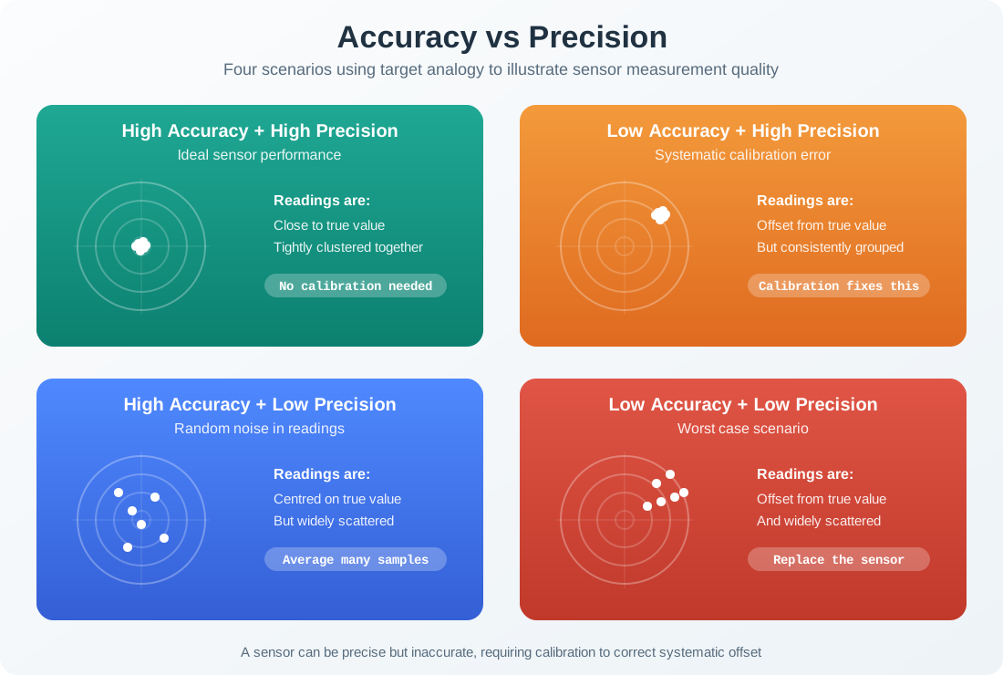
Intuition (the dartboard): precise but inaccurate is a tight cluster in the wrong place; accurate but imprecise is a loose scatter centred on the bullseye. They are different problems with different fixes — and neither is drift or hysteresis, which change over time or with direction.
Worked example: classify the mistake before fixing it
A temperature reference says the chamber is 25.0 °C. A sensor reports 27.9, 28.0, 28.0, 28.1, and 28.0 °C. The readings cluster tightly, so the sensor is precise. The cluster is about +3.0 °C from the reference, so it is inaccurate. Taking 100 more samples would make the mean look more stable, but it would still be near 28.0 °C unless you calibrate the offset.
Now suppose another sensor reports 24.4, 25.7, 24.9, 25.3, and 24.7 °C around the same reference. Its average is close to truth, but the spread is large for a control loop that needs stable tenth-degree changes. The fix is not the same. The first sensor needs calibration; the second needs noise reduction, bandwidth control, or a better front end. A third sensor that starts at 25.0 °C and creeps to 26.2 °C over a month has drift, so the fix is a recalibration interval. A pressure sensor that reads differently on the way up than on the way down has hysteresis, so you must test both directions.
Accuracy specifications often combine a fixed offset term with a proportional gain term. A meter specified as +/-(0.1% of input + 1 mV) over a 0 to 10 V input can be about +/-1 mV at zero, +/-6 mV near 5 V, and +/-11 mV near 10 V. The offset dominates near zero; the gain term grows with the signal. Keep both terms in the error budget instead of collapsing them into one headline percentage.
Co-located sensors give a useful precision test. Five temperature or humidity probes installed beside each other may trace the same weather pattern while small spreads, dropouts, and lag reveal repeatability, response, and installation differences. Agreement among the probes proves consistency within that group; it still needs a reference check before it proves absolute accuracy.
Overview Knowledge Check
24.5 Accuracy-Precision Confusion
Each confusion produces a predictable, costly mistake:
| The mistake | Why it fails |
|---|---|
| Averaging to improve accuracy | Averaging tightens random scatter (precision), but a systematic bias survives untouched — you get a very repeatable wrong answer. |
| Treating resolution as accuracy | A reading shown to five decimals can still be badly wrong; fine resolution does not imply closeness to truth. |
| Calibrate once, trust forever | Drift moves the response after calibration, so an old calibration slowly becomes wrong even if it was perfect on day one. |
| One-direction repeatability tests | Approaching a value only from below hides hysteresis, which only shows up when you also approach from above. |
Worked example: hysteresis hiding in a pressure sensor
A pressure sensor spanning 0–100 kPa is specified with 0.5% full-scale hysteresis. That means at a true 50 kPa the reading can differ by up to:
0.5% × 100 kPa = 0.5 kPa
…depending on whether you reached 50 kPa while pressure was rising or falling. A test that only ramps pressure upward will report excellent repeatability and completely miss this 0.5 kPa direction-dependent error.
Worked example: the wrong cure wastes the debug pass
A soil-moisture node gives ADC codes with a standard deviation of about 12 counts when the probe is held in one sample. Averaging 16 independent samples reduces random scatter by roughly sqrt(16) = 4, so the display noise may fall to about 3 counts. That is a precision improvement.
But if the probe was never calibrated and the conversion curve is shifted by 80 counts, the 16-sample average still carries almost the same 80-count bias. Likewise, if the reading changes by 20 counts after the probe sits in the soil for an hour, the issue may be settling or drift rather than random noise. The practical mistake is treating every bad reading as a filtering problem. Before writing more smoothing code, record whether the symptom is scatter, offset, slow change, direction dependence, clipping, or an impossible value.
This classification step also protects the rest of the troubleshooting checklist. A voltage-level mistake is solved before calibration, an address mistake is solved before filtering, and a warm-up mistake is solved before publishing data. The order matters because each unchecked mistake can make the next measurement look worse than it is.
Practitioner Knowledge Check
24.6 Different Errors Need Remedies
The reason the distinction matters is that each of the four has a different cure. Reach for the wrong cure and the error stays.
Accuracy → calibration
Close the gap to truth with a traceable reference. Averaging and higher resolution do nothing for a bias; only comparison against a known standard does.
Precision → averaging and bandwidth
Tighten random scatter by averaging uncorrelated samples, limiting bandwidth, and using a lower-noise front-end — the tools that do nothing for accuracy.
Drift → recalibration and tempco
Set a recalibration interval sized to tolerable drift, and compensate temperature coefficient in firmware if a temperature reading is available. A one-time calibration cannot hold back drift.
Hysteresis → hardware and characterisation
No fit removes path dependence; it must be minimised in the material/mechanics and then characterised by testing both directions and quoting it as residual uncertainty.
Worked example: build an error budget instead of trusting resolution
A tank-level sensor is displayed with 0.1 cm resolution, but the error budget is larger. Calibration against a ruler leaves a possible +0.4 cm bias. Repeat readings have random scatter of about 0.2 cm standard deviation. Averaging 16 samples reduces that random term to about 0.2 / sqrt(16) = 0.05 cm. The display looks steady, but the calibration term still dominates.
If the sensor drifts by 0.1 cm per month and the last calibration was six months ago, add another possible 0.6 cm. If filling and draining tests differ by 0.3 cm at the same level, hysteresis adds another residual uncertainty. A conservative worst-case statement is about 0.4 + 0.05 + 0.6 + 0.3 = 1.35 cm. A root-sum-square estimate would be smaller, but only if the assumptions about independent errors are justified.
The reporting mistake is to publish "level = 47.3 cm" with no context. A better engineering record says "47.3 cm, calibrated six months ago, random noise after averaging about 0.05 cm, drift allowance about 0.6 cm, hysteresis allowance about 0.3 cm." That record tells the next engineer whether to recalibrate, filter, change hardware, or simply accept the uncertainty.
The deepest mistake underneath all four is reporting a bare number with no sense of its error character. "23.7 °C" hides whether that carries a two-degree bias, hundredth-degree noise, an hourly drift, or a direction-dependent offset. And resolution never rescues the weakest link: a 24-bit ADC in front of a 2%-accurate sensor still gives a 2%-accurate result. A trustworthy reading always travels with its error budget.
Under-the-Hood Knowledge Check
24.7 Release Checklist
Before accepting a sensor reading, record these measurement-quality checks:
- Reference value and measured readings used to judge accuracy.
- Repeat-read spread used to judge precision or repeatability.
- Time, temperature, and environmental span used to judge drift.
- Rising and falling test paths used to judge hysteresis.
- Resolution, calibration age, random noise, drift allowance, and residual hysteresis in the reported uncertainty.
24.8 See Also
- Common Sensor Mistakes for the hardware and firmware mistake checklist.
- Sensor Specifications for accuracy, resolution, range, and response-time vocabulary.
- Sensor Noise and Averaging Limits for SNR and averaging boundaries.
- Sensor Calibration for offset, gain, and nonlinearity correction.
24.9 Next
Return to Common Sensor Mistakes once the error type is classified, then apply Sensor Calibration if the dominant error is bias, gain, or drift.