7 Choosing the Right Sensor

7.2 Field Conditions Drive Selection

Inspect Figure 7.1 to replace a product-photo decision with the actual deployment boundary and its field constraints.

Read Figure 7.1 from WET / SALINE ZONE, which creates the corrosion exposure requirement, to the battery service route, which sets maintainability and power constraints. The 80 m cable / radio path turns range and gateway margin into evidence rather than a datasheet-only claim.

The installation photograph ties those abstract constraints to the hardware at root depth: the probe body, tines, sealed cable gland, and burial-rated cable are all visible, so environmental fit can be reviewed against the real mounting boundary.

The mathematical gist. The chapter’s CR2477 exercise uses 0.070 mAh/day, or 2.92 µA, and a 1,000 mAh cell, giving 14,286 days before other losses. A catalog-typical 1% yearly self-discharge adds 1.14 µA. The total becomes 4.06 µA, so the same division gives 10,267 days, or 28.1 years. That result is arithmetic, not a promise: shelf aging and the microcontroller make the real life shorter.

Math Bridge · guided foundationsWhat does battery self-discharge do to 14,300 days?Let Phoebe turn capacity loss into current and recompute the chapter's CR2477 lifetime. Learn the maths

7.3 Prerequisites

• Sensor Specifications: Understanding key specs
• Common IoT Sensors: Available options

7.4 Introduction

With thousands of sensor models available, choosing the right one for a specific IoT project can feel overwhelming. A temperature sensor alone might have dozens of viable candidates across different technologies, price points, and form factors. Without a structured approach, teams often default to familiar sensors or the first result from an online search — only to discover months later that the sensor fails in deployment due to power, accuracy, environmental, or cost constraints they never evaluated.

This chapter presents a repeatable three-step methodology for sensor selection: define requirements, create a shortlist with a scored comparison matrix, and verify against datasheets. You will work through a complete outdoor deployment example, use interactive tools to explore how weighting priorities changes the “best” sensor, and study how Google’s Nest team navigated the transition from prototype sensor to production sensor at scale.

7.5 Stepwise Sensor Selection

Sensor selection is a structured engineering process, not guesswork. The following three steps transform vague project needs into a defensible sensor choice backed by data.

7.6 Sensor Selection Decision Tree

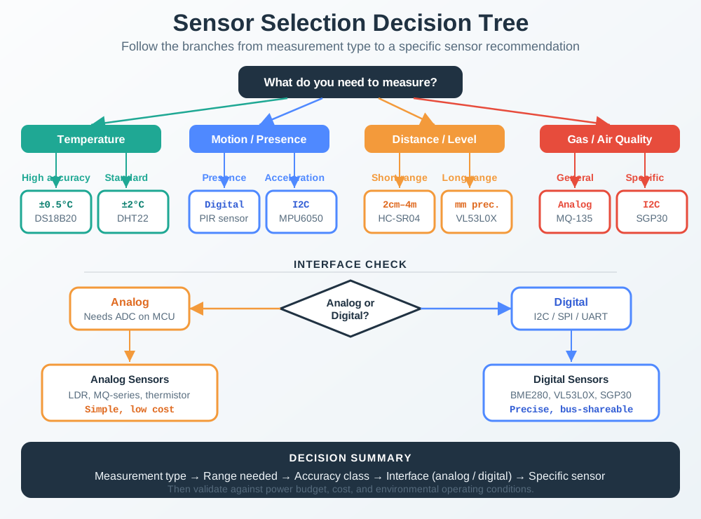
Figure 7.2 summarizes the three-step process as a visual flowchart. Start at the top with “What do you need to measure?” and follow the branches through accuracy, power, interface, and environment constraints to reach a recommended sensor.

Sensor selection decision tree from measurement type to recommended sensor

7.7 Quick Sensor Selector by Application

7.8 Outdoor Temp Choice

Requirements:

• Measure temperature -20C to +50C
• Accuracy +/-0.5C
• Battery-powered (2 years target)
• Read every 5 minutes
• Outdoor enclosure (IP65)
• Budget: $10 per sensor

Analysis:

Battery Life Calculation (DS18B20 sensor only):

• 288 readings/day x 0.75s x 1mA = 0.06mAh active
• 23.94 hours x 0.001mA = 0.024mAh sleep
• Total sensor consumption: 0.084mAh/day
• 2000mAh battery: 23,800 days (65 years theoretical, sensor only)

Note: This calculation covers only the sensor’s power draw. In practice, the microcontroller (ESP32, ATmega328P, etc.) dominates total power consumption. For example, an ESP32 in deep sleep draws approximately 10-150uA depending on configuration (RTC peripherals enabled, ULP coprocessor, etc.), adding 0.24-3.6mAh/day. Always calculate system-level power, not just sensor power, when estimating battery life.

Selection: DS18B20 - Best for outdoor due to waterproof probe option, excellent power efficiency, and meets accuracy requirement.

7.9 Automated Sensor Comparison

The key idea is weighted scoring: a sensor earns points for the requirements it satisfies, and high-priority requirements count more. Use the interactive weight explorer below first; the Python pattern is optional implementation detail.

weights = {
    "accuracy": 9,
    "waterproof": 10,
    "sleep": 7,
    "cost": 5,
    "humidity": 3,
}

candidates = {
    "DS18B20": ["accuracy", "waterproof", "sleep", "cost"],
    "DHT22": ["accuracy", "cost", "humidity"],
    "BME280": ["sleep", "cost", "humidity"],
}

def score(passed):
    earned = sum(weights[item] for item in passed)
    possible = sum(weights.values())
    return round(100 * earned / possible)

for sensor, passed in candidates.items():
    missing = set(weights) - set(passed)
    print(sensor, score(passed), "missing:", sorted(missing))

7.10 Budget Optimization Strategies

7.11 Nest Protect Sensor Selection

Sensor selection decisions that work at prototype scale can fail catastrophically at production volumes. The Nest Protect smoke and CO detector illustrates how production constraints reshape sensor choices.

Prototype phase (2012): Nest engineers initially prototyped with an MQ-2 gas sensor (the same $2 sensor common in hobbyist projects) alongside an optical smoke chamber. The MQ-2 performed well in lab tests — detecting smoke, CO, and natural gas.

Why MQ-2 failed at production scale:

Production solution: Nest selected a Figaro TGS5141 electrochemical CO sensor ($4.50 at volume) paired with a split-spectrum optical smoke chamber. The electrochemical sensor draws 0 mA at idle (no heater), responds within approximately 60 seconds (T90), maintains calibration for 10+ years, and distinguishes CO from other gases with near-zero cross-sensitivity.

The counterintuitive lesson: The production sensor cost 2x more per unit than the prototype sensor, but saved an estimated $12 per unit in battery costs (no heater = smaller battery), $8 per unit in warranty claims (fewer false alarms = fewer returns), and enabled the 6-year battery life that became a key selling point. Total cost of ownership was 40% lower despite higher sensor unit cost.

Checklist for prototype-to-production sensor transitions:

1. Calculate power budget over full product lifetime, not just active measurement
2. Verify sensor accuracy spec at end-of-life, not just new-from-factory
3. Test cross-sensitivity with realistic household interferents (cooking, cleaning products, humidity)
4. Confirm regulatory certification path (UL, CE, FCC) for the specific sensor model
5. Get volume pricing quotes — some sensors have steep quantity discounts, others do not
6. Evaluate supply chain risk — single-source sensors create production bottlenecks; consider dual-sourcing critical sensors or securing supplier agreements and safety stock to mitigate shortages
7. Request reliability data (MTTF) for the specific operating conditions of your product, not just the generic datasheet value

7.12 Concept Relationships

7.13 Sensor Fit Matrix Tradeoffs

The guide above shows the step-by-step selection workflow, scoring tools, and production checks. Continue to Sensor Selection Fit Matrices and Trade-Off Boundaries when you need the deeper L2 material: four-axis fit gates, auditable shortlist evidence, range-resolution trade-offs, response-time/noise trade-offs, and system-level error, power, timing, and maintenance budgets.

7.14 Summary

Key sensor selection takeaways:

Start with Define requirements first - Then find sensors, not the other way around. Then Create a shortlist - Compare 3-5 candidates systematically. Next Verify with datasheets - Don’t trust marketing specs alone. After that Consider total cost - Includes development time, libraries, support. Finally Prototype before production - Test in real conditions.

7.15 Try It Yourself

7.16 See Also

Start with Sensor Specifications - How to interpret accuracy, range, and power specs. Then Reading Datasheets - Extract requirements from sensor datasheets. Next Common IoT Sensors - Comparison of DHT22, DS18B20, BME280 options. Finally Common Mistakes - Avoid voltage mismatch and interface errors.

7.17 What’s Next

Now that you can select sensors using a structured methodology, explore these related topics: