28  Biomimetic Sensing

28.1 Start With the Measurement Story

Biomimetic sensing starts by asking what nature already solves well: detecting touch, vibration, chemicals, orientation, flow, or light under messy conditions. The engineering task is to borrow the principle, then prove it fits the device.

28.2 In 60 Seconds

Human skin contains 5 million sensors across five specialized receptor types, consuming only 10mW total. IoT designers can learn four key principles from this biological masterpiece: use multi-scale sensing (different sensors for different frequencies), implement adaptive response (slow-adapting for absolutes, fast-adapting for changes), build redundancy for graceful degradation, and process data hierarchically at the edge before sending to the cloud.

Phoebe’s Field Notes: The 50 Hz Filter Is Doing Real Nyquist Work

Phoebe’s Why

The “Hierarchical Bandwidth Savings” walkthrough later in this chapter treats the sensor-level step – “apply a 50 Hz low-pass filter and downsample from 1,000 samples/sec to 100 samples/sec” – as a bandwidth-and-cost move, which it is. It is also a textbook anti-alias filter, and it is worth naming as one: any time you throw away samples, whatever spectral content survives above the new, slower Nyquist limit does not disappear, it folds back down and disguises itself as a real low-frequency signal. Skin does the biological version of the same trick – Pacinian corpuscles are mechanically tuned to pass vibration and roll off the very-high-frequency content before it ever reaches a nerve fiber that fires far slower than the vibration itself. The engineering filter and the biological receptor are solving the identical folding problem.

The Derivation

A signal sampled at \(f_s\) has its spectrum replicated at every multiple of \(f_s\). Those images overlap the original band unless the signal is band-limited below half the sample rate:

\[f_s \geq 2f_{max} \quad\Longrightarrow\quad f_{max} = \frac{f_s}{2}\]

Any component above \(f_{max}\) does not vanish when sampled; it reappears at a folded (aliased) frequency \(|f - k f_s|\) for the nearest multiple \(k\), indistinguishable from a genuine low-frequency signal.

Worked Numbers: This Chapter’s Own 1,000 sps to 100 sps Pipeline

• Raw acquisition limit: this chapter’s own \(f_s = 1{,}000\) samples/s sets the analog front-end’s Nyquist ceiling at \(f_{max} = 500\) Hz – content above that must already be filtered before the ADC samples, or it aliases into the raw stream.
• Post-decimation limit: downsampling to this chapter’s own \(100\) samples/s drops the Nyquist ceiling to \(f_{max} = 50\) Hz.
• The filter is set exactly at the edge: this chapter’s own \(50\) Hz low-pass cutoff sits precisely at that new \(50\) Hz Nyquist limit, not below it with a guard band. A real single-pole (or even multi-pole) filter still passes meaningful energy right at its cutoff, so a machine with genuine vibration content near 45-55 Hz risks folding some of it into the decimated 100 sps stream. This is worth flagging as a design detail, not a documentation error: production systems usually set the anti-alias cutoff at a fraction of the new Nyquist limit (for example 30-40 Hz here) to leave a transition-band margin, which this walkthrough’s numbers do not show.
• Why it still works for the stated goal: the 333x bandwidth reduction this chapter reports is about discarding redundant slow machine-health trends, not resolving content near 50 Hz, so the tight margin is a reasonable engineering trade for that specific goal – it would not be reasonable if the application cared about vibration content near the cutoff itself.

28.3 Key Concepts

• Biomimetic Sensing: Design of artificial sensors inspired by biological sensory systems; examples include electronic noses (gas sensor arrays), artificial skin (tactile arrays), and whisker-based tactile sensors modeled on animal vibrissae
• Electronic Nose (e-Nose): An array of partially cross-selective gas sensors whose combined response pattern is analyzed with machine learning to identify complex odor mixtures, mimicking the mammalian olfactory system
• Neuromorphic Sensing: Sensor architectures inspired by biological neural processing where events are only triggered when the stimulus changes (like retinal ganglion cells), dramatically reducing data volume compared to frame-based cameras
• Tactile Sensor Array: A grid of pressure-sensitive elements measuring distributed force across a surface; used in robotic hands, prosthetics, and surface quality inspection; mimics receptor distribution in human skin
• Artificial Lateral Line: An array of pressure and flow sensors inspired by the fish lateral line organ; enables underwater robots to sense hydrodynamic disturbances and track moving objects without visual contact
• Compound Eye Camera: An imaging system using multiple small lenses covering a wide field of view, inspired by insect compound eyes; provides near-180 degree vision in an ultra-thin profile
• Bioinspired Signal Processing: Computational algorithms derived from biology, such as spiking neural networks for event-driven sensor data, providing energy efficiency by only computing in response to input changes
• Whisker Sensor: A flexible cantilever beam with strain gauges at the base, mimicking sensory whiskers of rodents; used on mobile robots for proximity and texture detection in low-visibility environments

Learning Objectives

After completing this chapter, you will be able to:

• Explain how human skin’s sensor architecture inspires IoT design
• Apply the four biomimetic design principles to sensor system design
• Design multi-scale sensing systems combining different sensor types
• Implement hierarchical data processing from edge to cloud
• Create redundant sensor systems that degrade gracefully

28.4 For Beginners: Biomimetic Sensing

“Biomimetic” means learning from nature. Your skin contains millions of tiny sensors that detect pressure, temperature, and texture, all while using incredibly little energy. Engineers study how biological systems sense the world to design better IoT sensor networks. For example, just as your skin uses different sensor types for different jobs, a smart building might use a mix of temperature, motion, and light sensors working together.

Chapter Roadmap

This chapter has five stops:

1. First you inspect skin as a reference design: 5 million receptors, 1.7 m², about 10mW.
2. Then you convert biology into four engineering principles: multi-scale sensing, adaptation, redundancy, and edge-before-cloud processing.
3. Next you test the ideas with BioTac, calculators, and the 333x processing example.
4. After that you stress-test event-driven designs with Observe rate limiting, quizzes, and project patterns.
5. Finally you review relationships, pitfalls, and the next sensor topics to study.

Checkpoints recap the design decisions; widgets carry the arithmetic.

28.5 Prerequisites

• Sensor Introduction: Basic sensor concepts and terminology
• Electronics Fundamentals: Understanding of analog and digital signals

28.6 Nature’s Perfect Sensor: Human Skin

Start with the biological baseline before choosing parts. Do not copy skin literally; notice how it uses structure, adaptation, redundancy, and local processing.

Before designing IoT sensors, consider the most sophisticated sensing system ever evolved: human skin. Understanding nature’s solution provides profound insights for engineering better sensor systems.

28.7 Lessons from Biology

Your skin contains approximately 5 million sensors packed into just 1.7 m² of “sensor array” that:

• Detects pressure from 0.1g to 10kg (100,000x dynamic range)
• Responds in 1-500ms (adapts to stimulus type)
• Consumes only ~10mW total (incredible energy efficiency)
• Self-heals and recalibrates continuously (no maintenance required)

This biological sensor network puts most IoT systems to shame in terms of efficiency, robustness, and adaptability.

28.8 Skin’s Multi-Scale Sensor Architecture

Human skin doesn’t rely on a single sensor type. Instead, it uses multiple specialized receptors working together—a principle directly applicable to IoT sensor design:

Figure 28.1: Human skin sensory structure: specialized receptors sit at different depths and respond to different touch, stretch, vibration, pain, and temperature signals

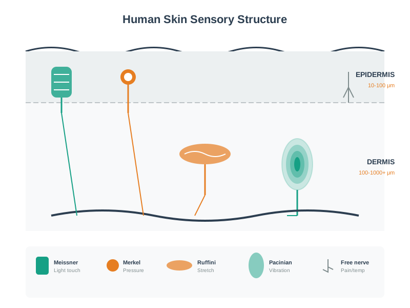
Mapping Biological Sensors to Engineering:

Skin Receptor	Sensation	Adaptation	Engineering Equivalent	Key Property
Merkel discs	Light touch, texture	Slow adapting	Strain gauge, pressure sensor	High spatial resolution (0.5mm)
Meissner corpuscles	Flutter, slip detection	Fast adapting	Vibration sensor (10-50 Hz)	Detects when objects slip from grasp
Pacinian corpuscles	Deep vibration	Very fast adapting	Accelerometer (50-500 Hz)	Maximum sensitivity at 200-300 Hz
Ruffini endings	Skin stretch, hand shape	Slow adapting	Strain sensor, force sensor	Directional sensitivity
Free nerve endings	Pain, temperature	Multi-modal	Thermistor, damage detector	Wide temperature range (~5°C to 50°C, with pain responses beyond)

Figure 28.2: Fast- and slow-adapting cutaneous mechanoreceptors divide dynamic light-touch events from sustained pressure and shape sensing

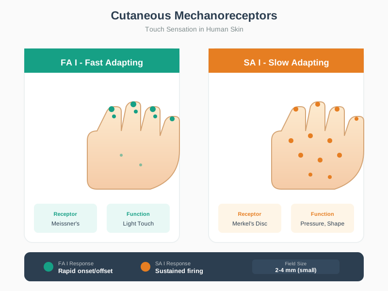Checkpoint: Skin as a Sensor Network

You now know:

• Skin combines about 5 million sensors across 1.7 m² instead of relying on one universal receptor.
• Different receptors cover different jobs: pressure, flutter, vibration, stretch, pain, and temperature.
• The benchmark is demanding: 0.1g to 10kg, 1-500ms response, and about 10mW total power.

28.9 Key Biomimetic Design Principles

Analyzing human skin reveals four critical principles for IoT sensor design:

28.9.1 Multi-Scale Sensing

Biological Insight: Skin uses different receptors for different frequency ranges (0.5 Hz to 500 Hz). No single receptor handles everything.

IoT Application:

• Don’t use one sensor type for all conditions
• Combine sensors with different response times:
  • Slow/static: Temperature (minutes), soil moisture (hours)
  • Medium/quasi-static: Vibration monitoring (1-10 Hz), door sensors
  • Fast/dynamic: Accelerometer (100+ Hz), acoustic sensors (kHz)

Real Example - Predictive Maintenance:

System combines three sensing scales:

• Slow thermal drift: Temperature sensor sampled once per minute.
• Medium mechanical change: Low-frequency vibration sampled around 10 Hz for bearing wear.
• Fast structural events: High-frequency accelerometer sampled around 1000 Hz for crack detection.

The useful insight is not the exact numbers; it is that one sensor stream cannot see every time scale.

28.9.2 Slow and Fast Sensor Adaptation

Biological Insight: Merkel discs (slow adapting) continuously report pressure, while Pacinian corpuscles (fast adapting) only respond to changes. This saves neural bandwidth.

A touch receptor also encodes more than “pressed” or “not pressed.” For a stronger indentation, the nerve fires a denser burst of spikes; as the stimulus becomes familiar, that pulse density decays. The engineering analogy is an event stream whose rate carries amplitude at the moment of change, while adaptation keeps a steady condition from consuming bandwidth forever.

IoT Application:

• Use slow-adapting (DC-coupled) sensors for absolute measurements:
  • Room temperature, water level, battery voltage
• Use fast-adapting (AC-coupled) sensors for change detection:
  • Motion sensors (PIR), vibration, acoustic events
• Energy savings: Fast-adapting sensors can sleep between events

Design Pattern - Adaptive Sampling:

Use two reporting paths instead of one constant stream:

• Slow path: read temperature on a schedule and publish the absolute value.
• Fast path: keep the camera asleep until motion or vibration crosses a threshold.
• Idle path: if nothing changes, return the node to deep sleep instead of transmitting “nothing happened.”

This is the engineering version of slow-adapting skin receptors reporting baselines while fast-adapting receptors report only changes.

28.9.3 Redundancy and Graceful Failure

Biological Insight: Skin has overlapping sensor coverage. Damage to one receptor type doesn’t cause total failure.

IoT Application:

• Sensor fusion: Combine multiple sensors for critical measurements
  • IMU = accelerometer + gyroscope + magnetometer
  • Indoor localization = Wi-Fi RSSI + BLE beacons + barometric altitude
• Fail-safe design: System continues with reduced accuracy if one sensor fails

Real Example - Autonomous Vehicles:

Redundant perception in practice:

• LiDAR: High-resolution primary distance sensing.
• Radar: Lower-resolution backup that still works in fog and rain.
• Camera: Context, color, signs, lanes, and object type.

If LiDAR fails, the vehicle should reduce speed and continue with radar plus camera rather than failing silently.

28.9.4 Edge-Before-Cloud Processing

Biological Insight: Significant signal processing occurs in nerve endings and spinal cord before reaching the brain. Only important signals trigger cortical attention.

Skin does not send all 5 million sensor readings to your brain — that would overwhelm the nervous system. Instead, processing happens in layers:

1. Receptor level — Mechanoreceptors convert pressure to electrical impulses (analog-to-digital conversion)
2. Peripheral nerve — First filtering: only significant changes pass through (edge detection)
3. Spinal cord — Pattern recognition: “Is this pain? Temperature change? Vibration?”
4. Thalamus — Data fusion: combines touch + temperature + pain into a unified sensation
5. Cortex — Conscious perception: only about 1% of original signals reach awareness

This yields a massive bandwidth reduction: 5M sensors at ~100 Hz produce ~500M signals/sec at the receptor level, yet only ~5M signals/sec reach the cortex (99% filtered locally).

IoT Application:

• Don’t send raw sensor data to cloud! Process locally:
  • Sensor level: Hardware filtering (RC circuits, op-amps)
  • Edge MCU: Thresholding, averaging, anomaly detection
  • Gateway: Data fusion, time-series compression
  • Cloud: Long-term analytics, model training

Quantified Impact — Smart Factory:

Raw to cloud

100 sensors at 1,000 samples/sec produce 100,000 readings/sec.

Stage 1: decimate

Hardware filtering reduces 100,000 readings/sec to 10,000 samples/sec.

Stage 2: edge filter

Discarding normal behavior reduces 10,000 samples/sec to 500 samples/sec.

Stage 3: compress and batch

Gateway processing reduces 500 samples/sec to about 150 messages/sec.

The result is a 99.85% reduction. At $0.50 per million messages, the monthly ingestion cost drops from about $129,600 to about $194.

Checkpoint: Four Design Principles

You now know:

• Multi-scale sensing separates slow, medium, and fast phenomena instead of forcing one stream to do every job.
• Fast-adapting channels report changes; slow-adapting channels preserve absolute state.
• Redundancy and edge-before-cloud processing keep systems useful when one sensor fails or raw data volume is too high.

28.9.5 Processing Savings Calculator

Use this calculator to estimate the bandwidth and cost savings from applying biomimetic hierarchical processing to your IoT sensor deployment.

Number of sensors Sample rate (Hz) Bytes per sample Decimation factor Edge filter percentage Gateway compression ratio Cloud cost ($/million messages)

28.10 Skin-to-IoT Design Framework

Use these biomimetic principles when designing your next IoT sensor system. The diagram below maps biological processing layers to their IoT equivalents:

Figure 28.3: Biomimetic vs IoT layered processing architecture comparison

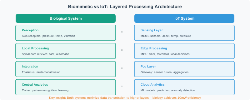
This layered view emphasizes the hierarchical processing architecture shared by biological and IoT sensing systems. Both systems minimize data transmission to higher layers by processing locally — biology achieves a remarkable 10mW power budget that IoT systems strive to approach.

28.11 SynTouch BioTac Tactile Sensor

SynTouch, a Los Angeles company spun out of the University of Southern California’s biomechanics lab, commercialized the BioTac sensor in 2012 — one of the most faithful engineering reproductions of human fingertip sensing. The BioTac demonstrates all four biomimetic principles in a single $5,000 sensor module.

How it mimics skin architecture:

Human Skin Feature	BioTac Implementation	Sensing Capability
Dermal ridges (fingerprints)	Silicone elastomer skin with molded ridges	Texture discrimination (117 materials at 95% accuracy)
Merkel discs (slow adapting)	DC pressure electrode array (19 impedance sensors)	Static force measurement (0.01-10 N range)
Pacinian corpuscles (fast adapting)	Hydrophone pressure sensor in fluid core	Vibration detection (up to 1,000 Hz)
Thermoreceptors	NTC thermistor embedded in rigid core	Temperature sensing and thermal conductivity (metal vs. plastic vs. wood)
Interstitial fluid	Incompressible liquid filling the elastomer	Distributes force uniformly across all sensors

Multi-scale sensing in practice:

The BioTac achieves what no single-principle sensor can: simultaneous measurement of force (DC), vibration (AC), temperature, and texture from a single 25 mm fingertip-sized package. When a robot hand grasps an object:

1. DC electrodes detect initial contact force and grip pressure (0-50 Hz, Merkel-like)
2. Hydrophone detects micro-slip vibrations indicating the object is about to fall (100-1,000 Hz, Pacinian-like)
3. Temperature sensor identifies material type by thermal conductivity (metal feels cold, wood feels warm)
4. All combined: The robot adjusts grip force in real-time, using less force for delicate objects and more for heavy ones — exactly how your hand works

Real-world deployment — Shadow Dexterous Hand:

Shadow Robot Company (London) integrated BioTac sensors into their five-fingered robotic hand for pharmaceutical laboratory automation. According to SynTouch case studies, reported results from pilot deployments include:

• Vial handling success rate: ~99.7% (vs. ~94% without tactile feedback) — the BioTac detected micro-slips approximately 50 ms before visible movement
• Breakage reduction: Up to 85% fewer broken glass vials (the sensor detected excessive grip force and reduced it)
• Material sorting: Correctly identified 15 different vial cap materials by thermal signature alone, enabling automated sorting that previously required visual inspection

Cost-effectiveness analysis:

The BioTac costs $5,000 per sensor — expensive for consumer products but justified in high-value applications. At the pharmaceutical company, each broken vial of compound cost $2,000–$15,000 in wasted material. Preventing just 4 vial breaks per month ($8,000–$60,000 saved) justified the $50,000 investment in BioTac sensor upgrades (10 fingertip sensors for existing robot hands) within 1–6 months.

Design lesson: You do not need to implement all biomimetic principles simultaneously. SynTouch’s key insight was that the liquid-filled core (mimicking interstitial fluid) was the critical innovation — it converts any local pressure into a distributed signal that all 19 electrodes can detect. This single design decision enabled multi-scale sensing from a mechanically simple structure. When applying biomimetic principles, identify the one biological mechanism that enables the broadest sensing capability, and build your design around it.

Checkpoint: From Principle to Product

You now know:

• The BioTac packages force, vibration, temperature, and texture in one 25 mm sensor.
• Its 19 impedance sensors and fluid core turn local pressure into distributed evidence.
• A $5,000 sensor can make sense when it prevents $2,000–$15,000 vial losses and cuts breakage by up to 85%.

28.12 Biomimetic Design Checklist

Use this checklist when designing your sensor systems:

• Multi-scale sensing: Do I have sensors for different time scales (slow DC + fast AC)?
• Adaptive response: Can fast-changing sensors sleep between events?
• Redundancy: What happens if my primary sensor fails?
• Hierarchical processing: Am I processing data at the edge before sending to cloud?
• Energy budget: Have I calculated total power consumption (skin uses only 10mW for 5M sensors)?

28.12.1 Sensor Power Budget Estimator

Compare your IoT sensor system’s energy efficiency against the biological benchmark of human skin (10mW for 5 million sensors = 2 nW per sensor).

Number of IoT sensors Power per sensor (mW) Duty cycle (%) Battery capacity (mAh) Battery voltage (V)

28.13 Hierarchical Bandwidth Savings

Scenario: A predictive maintenance system monitors 200 industrial machines with vibration sensors. Each sensor produces 1,000 samples/second (16-bit ADC values).

Without edge processing (raw data to cloud):

• Each sensor generates 2 KB/s: 1,000 samples/sec times 2 bytes.
• Across 200 sensors, the raw stream is 400 KB/s.
• That becomes about 34.56 GB/day and roughly 1 TB/month.
• If each sample is sent as a cloud message, ingestion reaches 518.4 billion messages/month, or about $259,200/month at $0.50 per million messages.

With hierarchical edge processing (biomimetic approach):

1. Sensor level: apply a 50 Hz low-pass filter and downsample from 1,000 samples/sec to 100 samples/sec.
2. Edge MCU: discard normal behavior, send summaries during steady operation, and send short bursts only around anomalies.
3. Gateway: compress the time-series and batch summaries before cloud upload.

The final cloud stream is about 1.2 KB/s, or 3.11 GB/month. Bandwidth drops from 1,037 GB/month to 3.11 GB/month, and message cost drops from about $259,200/month to about $778/month.

28.14 Putting Numbers to It

Hierarchical processing mirrors biological filtering. Raw data rate without edge processing:

\[\text{Rate} = 200 \text{ sensors} \times 1{,}000 \text{ samples/s} \times 2 \text{ bytes} = 400{,}000 \text{ bytes/s}\]

Monthly volume: \(400 \text{ KB/s} \times 86{,}400 \text{ s/day} \times 30 \text{ days} = 1{,}036{,}800{,}000 \text{ KB} \approx 1{,}037 \text{ GB/month}\)

With 3-stage filtering, the combined reduction is about 333x. The final rate is about 1.2 KB/s, or 3.11 GB/month. AWS cost drops from $259,200/month to $778/month, a monthly savings of about $258,422.

Key insight from biology: Just as skin receptors filter 99% of stimuli before reaching the spinal cord (only pain and significant changes trigger cortical attention), IoT systems should process locally and send only actionable insights to the cloud.

28.15 DC vs AC Sensor Adaptation

When designing an IoT sensor node, one of the first architecture decisions is whether to use slow-adapting (DC-coupled) or fast-adapting (AC-coupled) sensors. This table helps match sensor type to application requirements:

Requirement	Use Slow Adapting (DC)	Use Fast Adapting (AC)
Measure absolute value	Temperature monitoring (need to know it’s 22.5°C, not just “changed by 0.5°C”)	No: not suitable
Detect changes/events	No: wasteful because it sends a constant stream	Motion detection (PIR), door open/close, vibration alerts
Battery-powered with multi-year target	Only if reading interval > 1 hour	Yes: ideal for sleeping between events and improving battery life
Continuous monitoring required	Yes: required for medical vitals and HVAC control	No: would miss baseline drift
High-frequency sampling (>100 Hz)	No: wasteful bandwidth	Yes: accelerometer for crack detection; send only when vibration exceeds threshold
Legal/compliance requirement for absolute values	Yes: required for FDA medical devices or custody-chain temperature logs	No: cannot prove absolute state

Hybrid approach example - Smart thermostat:

• Baseline report: publish the absolute room temperature every 5 minutes.
• Event report: publish an immediate alert when temperature changes by more than 2°C in 10 seconds.
• Why both: the baseline supports HVAC control and records; the event path catches abnormal events quickly without streaming every sample.

Decision rule: Default to fast-adapting (AC) for battery-powered devices unless absolute values are legally/functionally required. Hybrid systems use both: AC for real-time alerts, DC for periodic baseline reporting.

28.16 Rate-Limited Observe Patterns

The Error: A smart factory deployed 1,000 CoAP sensors using the Observe extension for real-time monitoring. Each sensor had 3 dashboard clients observing its vibration data (3,000 total subscriptions). During a machine malfunction, vibration values changed 50 times/second, generating 150,000 notifications/second (1,000 sensors × 3 observers × 50 changes/s). The network collapsed within 90 seconds.

Why it happened: The Observe extension (inspired by fast-adapting biological receptors) pushes every change to all subscribers. Without server-side rate limiting, rapidly-changing sensor values trigger notification floods. The engineers assumed “server push is efficient” without considering burst traffic.

The fix - Implement server-side rate limiting:

Use two gates before notifying observers:

1. Change gate: skip the update unless the value changed by at least 10%.
2. Time gate: skip the update if the same observer received a notification less than 500 ms ago.
3. State update: when both gates pass, send the notification and remember the last value and time for that observer.

This keeps the biological idea of event-driven sensing while preventing notification storms during abnormal conditions.

Real impact numbers:

• Before fix: 150,000 notifications/s → 500 Mbps network saturation → system crash
• After fix: 6,000 notifications/s (500ms rate limit) → 20 Mbps → stable operation
• Biological parallel: Pacinian corpuscles in skin adapt within 50ms, preventing saturation of neural pathways. The fix mimics this biological rate-limiting behavior.

Prevention: Always implement MIN_NOTIFY_INTERVAL and CHANGE_THRESHOLD for Observe/subscribe patterns. Test with worst-case change rates (machine startup, anomaly conditions) during development, not just steady-state operation.

Checkpoint: Rate-Limited Edge Evidence

You now know:

• Raw hierarchical processing can drop 200 sensors at 1,000 samples/second from about 1 TB/month to 3.11 GB/month.
• The 333x reduction and $259,200/month to $778/month cost drop only work when filtering is staged locally.
• Event-driven Observe systems still need rate limits: 150,000 notifications/s collapsed the network, while 500 ms gating held it to 20 Mbps.

28.17 Label the Diagram

28.18 Code Challenge

28.19 Piezo Touch Dynamics

The body above introduces biomimetic sensing as a design pattern across skin-like receptor types, adaptation, redundancy, and edge processing. Continue to Piezoelectric Touch and Dynamic Biomimetic Sensing when the design question is specifically about fast-adapting tactile or vibration channels. That page separates the deeper material: piezoelectric charge generation, charge-amplifier sizing, low-frequency cutoff, leakage, and why a dynamic piezo channel needs a static-capable partner.

28.20 Engineering Lessons from Skin

The human skin sensor system represents 500 million years of evolutionary optimization. Key takeaways for IoT design:

1. No universal sensor: Use specialized sensors for different tasks (just like skin has 5+ receptor types)
2. Energy efficiency: Skin’s 10mW for 5M sensors proves hierarchical processing works
3. Adaptation matters: Fast-adapting sensors save bandwidth by reporting only changes
4. Redundancy is essential: Overlapping sensor coverage provides robustness
5. Process locally: Brain doesn’t analyze every nerve impulse; cloud shouldn’t analyze every sensor reading

28.21 Biomimetic Design Principles

28.22 Touch-Sensitive LED Strip

Goal: Create a light strip that responds to touch using capacitive sensing (mimics Merkel discs).

Components:

• ESP32 (has built-in capacitive touch pins)
• LED strip (WS2812B)
• Aluminum foil or copper tape (touch electrodes)

Behavior to implement:

• Touch left electrode: LEDs shift left
• Touch right electrode: LEDs shift right
• Touch both: Change color
• Release: Fade out

Biomimetic principle: Fast-adapting response (only triggers on touch/release, not continuous pressure)

28.23 Multi-Scale Vibration Monitor

Goal: Implement Pacinian-like sensing with different frequency bands.

Hardware:

• ADXL345 accelerometer (high-frequency capable, up to 3200 Hz)
• Three frequency bands:
  • Slow (0.5-10 Hz): bearing wear
  • Medium (10-100 Hz): motor imbalance
  • Fast (100-1000 Hz): crack formation

Algorithm:

1. Sample at 3200 Hz
2. Apply band-pass filters (digital IIR)
3. Calculate RMS power in each band
4. Trigger alerts per band

Biomimetic parallel: Just like skin has Merkel (slow), Meissner (medium), Pacinian (fast) receptors

28.24 Tactile Feedback Gripper

The three mini-projects above turn the chapter into implementation choices: capacitive touch, band-pass vibration, and force plus piezo slip control.

Goal: Build a gripper that detects object slip before it falls (mimics Meissner corpuscles).

Sensors:

• Force-sensitive resistors (FSR) for grip pressure (slow-adapting, like Ruffini)
• Piezo vibration sensors for slip detection (fast-adapting, like Meissner)

Control algorithm:

1. Grip object with initial force F
2. Monitor vibration sensor (10-50 Hz band)
3. If vibration spike detected → increase grip force by 10%
4. If force > max safe threshold → alert “object too heavy”

Challenge: Prevent crushing delicate objects while preventing slips

28.25 Concept Relationships

Core Concept	Related Concepts	Why It Matters
Multi-Scale Sensing	Frequency Bands, Specialized Sensors	No single sensor handles all conditions
Adaptive Response	Fast vs Slow Adapting, Event Detection	Saves bandwidth by reporting only changes
Hierarchical Processing	Edge Filtering, Gateway Fusion, Cloud Analytics	Reduces data transmission by 99%+
Redundancy	Sensor Fusion, Graceful Degradation	System continues with reduced accuracy if sensor fails

Common Pitfalls

28.25.1 Biomimetics Are Not Drop-Ins

Biomimetic sensors produce raw data in very different formats — an e-nose produces multi-channel resistance vectors, not a single concentration value. Processing requires pattern recognition algorithms, not simple threshold comparisons. Plan for the additional signal processing complexity before committing to this sensor class.

28.25.2 E-Nose Training Data Gaps

Electronic nose systems rely on machine learning models trained on labeled sensor responses. A model trained at one temperature and humidity may fail in different conditions. Collect training data across the full range of expected deployment conditions, not only in controlled lab settings.

28.25.3 Tactile Array Calibration Gaps

Individual elements in a tactile array have manufacturing variations of +-5-20%. Treating all elements as identical causes systematic errors in force mapping. Calibrate each element individually before deploying the array for quantitative force measurement.

28.25.4 Neuromorphic Timing Dependencies

Event-driven sensors produce asynchronous event streams where meaning depends on precise timing relative to other events. Standard frame-based pipelines cannot handle this format correctly. Ensure your data acquisition architecture natively supports asynchronous timestamped event streams.

28.26 What’s Next

With biomimetic design principles in hand, explore these related topics to deepen your sensor system expertise:

Topic	Link	Why It Matters
Piezoelectric Touch	Piezoelectric Touch and Dynamic Biomimetic Sensing	Size fast-adapting tactile channels and pair them with static pressure sensing
Sensor Specifications	Accuracy, response time, and range	Translate biomimetic principles into quantified sensor requirements
Signal Processing	Filtering and noise reduction	Implement the hierarchical edge-filtering techniques covered here
Common IoT Sensors	Popular sensors and MEMS technology	Select real hardware that maps to the multi-scale sensing approach
Sensor Calibration	Calibration techniques and drift	Maintain accuracy over time — biology self-calibrates, IoT must be calibrated manually
Edge Computing	Processing at the edge	Scale hierarchical processing from single nodes to distributed architectures

Continue to Sensor Specifications ->