12 Bridge Linearity and Instrumentation
12.1 Start With the Measurement Story
A bridge circuit can reveal a tiny physical change, but only if the weak differential signal survives imbalance, noise, and loading. Start by following the signal from bridge output through instrumentation gain to an ADC-ready value.
12.2 Learning Objectives
After this page, you should be able to:
- Explain why bridge circuits cancel large sensor baselines before amplification.
- Estimate quarter-bridge output voltage from gauge factor, strain, and excitation voltage.
- Choose instrumentation-amplifier gain from the worst-case differential signal and ADC range.
- Use common-mode rejection and dummy gauges to suppress cable noise and thermal drift.
12.3 After Signal Conditioning
Signal Conditioning for Sensors introduces the full chain from physical sensor output to ADC-ready voltage. This page narrows in on bridge sensors, where the useful signal is often a few millivolts riding on a much larger baseline.
Use it when a strain gauge, load cell, pressure transducer, torque sensor, or other bridge sensor needs a readout that will not clip, waste ADC range, or treat temperature and cable noise as real motion.

Phoebe’s Why
This chapter states “GF (gauge factor) ~= 2.0 for metal foil” and moves straight to the bridge math, but that 2.0 is not an arbitrary calibration constant – it comes from two separate physical effects stacking up inside a single stretched wire. Stretch a resistive foil and its resistance changes for a purely geometric reason: it gets longer (more resistance) and, because the material barely changes volume, thinner (also more resistance). But most metals also change resistivity itself under strain, a genuine material property called the piezoresistive effect. Gauge factor is nothing more than the sum of those two contributions, and for a foil gauge alloy like constantan the geometric term does most of the work.
The Derivation
Starting from \(R=\rho L/A\) and differentiating:
\[\frac{dR}{R} = \frac{d\rho}{\rho} + \frac{dL}{L} - \frac{dA}{A}\]
Axial strain is \(\varepsilon = dL/L\). Poisson’s ratio \(\nu\) sets the matching transverse contraction (\(dr/r=-\nu\varepsilon\) for a round conductor), so the cross-section shrinks as \(dA/A=2\,dr/r=-2\nu\varepsilon\). Substituting:
\[\frac{dR}{R} = \frac{d\rho}{\rho} + \varepsilon - (-2\nu\varepsilon) = \frac{d\rho}{\rho} + \varepsilon(1+2\nu)\]
Dividing by strain defines the gauge factor as geometric plus piezoresistive terms:
\[GF = \frac{dR/R}{\varepsilon} = \underbrace{(1+2\nu)}_{\text{geometric}} + \underbrace{\frac{d\rho/\rho}{\varepsilon}}_{\text{piezoresistive}}\]
Worked Numbers: Decomposing This Chapter’s GF = 2.0
- Geometric term, using \(\nu\approx0.30\) (catalog-typical for constantan-type foil alloys): \(1+2(0.30)=1.60\) – length and thinning together already account for most of the chapter’s GF = 2.0 before any material effect is added.
- Piezoresistive remainder: \(2.00-1.60=0.40\), so about \(0.40/2.00=20.0\)% of this chapter’s gauge factor comes from constantan’s resistivity actually changing under strain, and 80.0% is pure geometry – which is exactly why a foil gauge is described as a mechanical-to-geometric sensor first and a resistivity sensor second.
- Recomputing this chapter’s own 1000 microstrain example from the decomposed terms: at \(\varepsilon=0.001\), the geometric contribution to \(\Delta R/R\) is \(1.60\times0.001=1.60\times10^{-3}\) and the piezoresistive contribution is \(0.40\times0.001=4.00\times10^{-4}\); summed, \(\Delta R/R=2.00\times10^{-3}\), matching \(GF\times\varepsilon\) exactly, and \(V_{out}=5.0\times2.00\times10^{-3}/4=2.50\) mV – the same 2.5 mV this chapter’s own worked example already states.
- Cross-check against the Practitioner Knowledge Check’s 500 microstrain case: \(\Delta R/R=2.00\times0.0005=1.00\times10^{-3}\), \(V_{out}=5.0\times1.00\times10^{-3}/4=1.25\) mV, matching the quiz’s own “About 1.25 mV” answer – confirming the decomposition reproduces every number this chapter already uses, not just the headline one.
12.4 Tiny Signals on Large Baselines
Some of the most useful sensors move only a whisker. A metal-foil strain gauge changes its resistance by roughly one part in a thousand at full mechanical load. If you drop that gauge into a plain voltage divider, the tiny wanted change rides on top of a large, steady baseline voltage — like trying to see a ripple on the surface of a full bathtub. The ADC spends almost all its range on the baseline and almost none on the signal.
Two classic building blocks solve this together. The Wheatstone bridge subtracts a matched reference so that, at rest, the output is zero and only the change appears as a small differential voltage. The instrumentation amplifier then amplifies that small differential voltage by a large, precise factor while rejecting interference that is common to both wires.
Intuition: the bridge is two voltage dividers side by side. Read the difference between their midpoints. When the arms are balanced the difference is zero, so you have thrown away the baseline and kept only the signal — before you amplify.
For a concrete feel, compare two ways to read a 350 Ω strain gauge excited from 5 V. In a single divider with another 350 Ω resistor, the midpoint sits near 2.500 V. A 0.1% resistance change moves that midpoint by only about 1.25 mV, so a 12-bit, 3.3 V ADC sees roughly 1.6 counts of movement on top of a 3100-count baseline. The bridge produces the same millivolt-scale change as a signed differential output around zero, which an instrumentation amplifier can safely multiply before the ADC. With gain 200, that 1.25 mV becomes 250 mV, or about 310 ADC counts. The measurement did not become more physically sensitive; the circuit simply stopped wasting ADC range on the baseline.
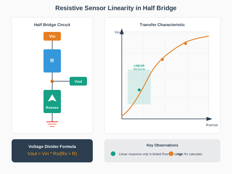
Linearize around the operating point
A simple half-bridge divider is not globally linear. Its midpoint voltage follows:
Vout = Vin * Rs / (Rs + R)
Rs = R0 + DeltaR
Near the chosen operating resistance R0, the first Taylor term is the sensitivity you want; the terms after it are the non-linear error you must bound:
V(Rs) ~= V(R0)
        + DeltaR * [dV/dRs at R0]
        + (DeltaR^2 / 2) * [d2V/dRs2 at R0] + ...
Datasheets often report nonlinearity as a percentage of full-scale output: the vertical error between the actual curve and the selected straight-line fit over the declared span. As |DeltaR| grows relative to R + R0, the quadratic and higher-order terms stop being negligible. The remedy is to keep the useful range near the matched operating point, use a bridge topology that cancels the baseline, or calibrate the curve instead of trusting one slope across the whole span.
Overview Knowledge Check
12.5 Quarter-Bridge Amplifier Sizing
With one active gauge (a quarter-bridge) and the other three arms fixed at the nominal resistance, the bridge output for a small change is approximately:
Vout / Vex ≈ (1/4) × (ΔR / R)

and for a strain gauge:   ΔR / R = GF × ε
  GF = gauge factor (≈ 2.0 for metal foil)
  ε  = strain (dimensionless, often quoted in microstrain)
Worked example: 1000 microstrain on a foil gauge
Given: strain ε = 1000 µε = 0.001
       gauge factor GF = 2.0
       excitation Vex = 5.0 V

Fractional change:  ΔR/R = 2.0 × 0.001 = 0.002 (0.2%)
Bridge output:      Vout = 5.0 × 0.002 / 4 = 2.5 mV

2.5 mV is far too small for a 3.3 V ADC to resolve well.
Amplify with an instrumentation amp at gain 100:
       Vout' = 2.5 mV × 100 = 250 mV   (now comfortably readable)
A real part makes the gain concrete. The AD620 instrumentation amplifier sets its gain with one external resistor: G = 1 + 49.4 kΩ / RG. For a gain of 100 you solve RG = 49.4 kΩ / 99 ≈ 499 Ω, which is a standard value the datasheet itself lists.
Ratiometric bonus: the bridge output is proportional to the excitation Vex. If the ADC reference is derived from the same Vex, drift in the excitation cancels in the reading — the same ratiometric idea that helps a plain divider, now applied to the bridge.
Keep the amplifier range honest before choosing the gain resistor. If the same load cell can see 1500 microstrain in an overload test, the raw output is 5.0 V × (2.0 × 0.0015) / 4 = 3.75 mV. Gain 100 produces 375 mV, leaving plenty of headroom. Gain 1000 produces 3.75 V, which clips a 3.3 V ADC and hides the overload exactly when you need evidence. A practical design therefore picks a gain from the worst-case signal, not just the nominal signal, then uses calibration coefficients to convert ADC counts back to force or pressure.
Practitioner Knowledge Check
12.6 CMRR and Thermal Cancellation
The bridge-plus-instrumentation-amp pairing is not just about gain. It is about rejecting everything you did not mean to measure.
Differential vs common-mode
The wanted signal is the difference between the two bridge midpoints. Interference — supply ripple, mains hum picked up on the cable — tends to appear equally on both, as a common-mode voltage.
The instrumentation amp's job
It amplifies the difference and rejects the common-mode part. A good in-amp rejects common-mode by a factor of 100,000 or more (over 100 dB), so shared noise is suppressed while the differential signal is amplified.
High input impedance
Its inputs draw almost no current, so the amplifier does not load and unbalance the bridge — a problem a simple op-amp stage with modest input resistance would cause.
Thermal cancellation
Temperature also changes gauge resistance. Placing a dummy, unstrained gauge in an adjacent bridge arm makes that thermal shift appear on both arms, so it cancels in the difference while real strain does not.
A quick noise budget shows why common-mode rejection matters. Suppose the real bridge signal is 2 mV, but a nearby motor couples 100 mV of 50 Hz noise equally onto both sensor wires. With a plain single-ended amplifier at gain 100, the noise would try to become 10 V and would slam the output into a rail. With an instrumentation amplifier whose common-mode rejection ratio is 100 dB, the common-mode component is reduced by a factor of 100,000 before the differential gain matters: 100 mV becomes about 1 µV equivalent input. After gain 100, that is only about 0.1 mV at the output, while the wanted 2 mV differential signal becomes 200 mV.
Thermal effects need the same differential thinking. A foil gauge might change resistance from both strain and temperature. If the active gauge rises by 0.20% from strain and both the active and dummy gauges rise by 0.05% from temperature, the bridge subtracts the shared thermal term and leaves the strain term as the dominant differential change. If the dummy gauge is mounted far from the active gauge, that assumption fails; the bridge then reports temperature gradients as fake mechanical load.
This is why load cells, pressure transducers, and torque sensors almost universally use a bridge feeding an instrumentation amplifier: the topology cancels the baseline, cancels temperature drift through matched arms, rejects common-mode interference, and keeps high source impedance from being disturbed, leaving a clean amplified copy of the mechanical signal.
Under-the-Hood Knowledge Check
12.7 Release Checklist
Before relying on a bridge-sensor readout, confirm these points:
- The bridge excitation voltage is within the sensor manufacturer’s self-heating and accuracy limits.
- The expected maximum strain, load, or pressure is converted into a worst-case millivolt bridge output.
- Instrumentation-amplifier gain leaves ADC headroom for overloads, offset, startup transients, and noise.
- The ADC reference and bridge excitation are intentionally ratiometric or independently stabilized.
- Cable shielding, twisted pairs, and amplifier layout preserve the common-mode rejection assumed in the calculation.
- Dummy or matched bridge arms see the same temperature as the active sensing element when thermal cancellation is expected.
12.8 See Also
- Signal Conditioning for Sensors for the full amplification, filtering, and ADC chain.
- Resistive Dividers and ADC Loading for single-ended resistive sensors before bridge circuits are needed.
- Sensor Data Processing for filtering and calibration after the bridge signal reaches firmware.
- Accuracy, Precision, Drift, and Hysteresis for reporting remaining uncertainty after conditioning.
12.9 Next
Return to Signal Conditioning for Sensors once the bridge gain and noise budget are clear, then continue to Sensor Data Processing for digital filtering and calibration.