41 Sensor Noise and Averaging Limits
41.1 Start With the Measurement Story
Noise averaging only helps when the signal story is understood. Begin by separating random noise from drift and interference, then use SNR and repeated samples to prove whether averaging improves the measurement enough.
41.2 Learning Objectives
After this page, you should be able to:
- Identify thermal, flicker, and ADC quantization noise in sensor front-ends.
- Estimate whether front-end noise, ADC step size, sensor tolerance, or environment dominates the error budget.
- Explain why averaging improves white noise but not slow drift or fixed bias.
- Choose between averaging, bandwidth limiting, shielding, grounding, reference checks, and calibration.
- Record enough evidence to defend a sensor reading as signal plus uncertainty rather than a single unqualified number.
41.3 After Sensor Lab Best Practices
Sensor Lab Best Practices teaches the defensive workflow: validate readings, filter noise, fuse sensors, monitor health, and use hysteresis. This page explains when those safeguards work and when they only hide the wrong failure mode.
Use it before adding larger averaging windows, changing thresholds, or declaring a sensor healthy. If variation is random and fast, bandwidth limiting and averaging can help. If the value drifts, moves with supply voltage, changes with placement, or disagrees by a fixed offset, the answer is evidence, calibration, or hardware cleanup rather than more samples.
41.4 Overview: Every Reading Comes With Noise
No sensor reading is perfectly still. Even with the input held constant, the value wobbles because of physical noise that no design can remove entirely, only manage. Good lab practice is really about managing the ratio between the signal you want and the noise you cannot avoid — the signal-to-noise ratio (SNR).
Three fundamental noise sources set the floor for most sensor front-ends. Thermal (Johnson) noise is the hiss produced by any resistance simply because it is warm. Flicker (1/f) noise grows as frequency falls, so it dominates slow, near-DC measurements. Quantization noise is the rounding error introduced by the ADC. Real circuits can add capacitive or inductive pickup, shot noise in junctions, and amplifier voltage or current noise on top of those floors. Knowing which one limits you tells you which fix will actually help.
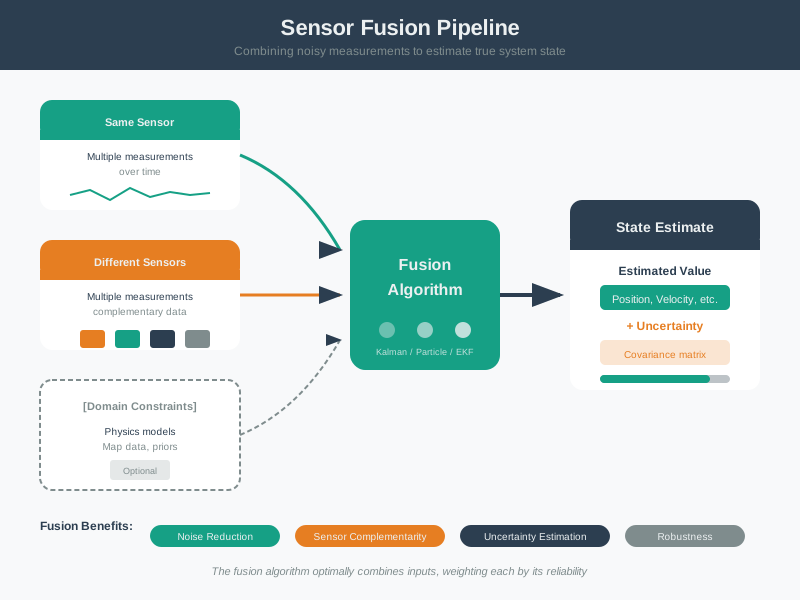
Intuition: you can raise SNR two ways — make the signal bigger (more gain, more excitation, better placement) or make the noise smaller (narrower bandwidth, averaging, lower-noise parts). Both matter, and the best design uses both.
This is why best-practice sensor logs record conditions, not just values. A temperature reading of 24.8 °C is more useful when the log also states the sensor model, sample interval, enclosure state, airflow, supply voltage, and whether the reading is raw, filtered, or calibrated. Without that context, a later reviewer cannot tell whether a 0.4 °C change is a real environmental shift or a power-rail, placement, or averaging artifact.
Noise work also decides when more code will not help. If the signal itself is small because the sensor is mounted too far from the phenomenon, averaging only hides the weak placement. If the ADC input is picking up motor switching spikes, a software moving average may smear the spike into several samples; the real fix is grounding, shielding, RC filtering, or sampling away from the switching edge. Lab discipline means changing one variable at a time and keeping enough evidence to explain why the fix worked.
Overview Knowledge Check

Phoebe’s Why
The Overview above names quantization as one of three noise floors, but the thermal-noise worked example never puts a number on it – so it looks smaller than it is. An ADC never reports the true analog voltage; it reports the code whose center is closest, and it rounds every value inside a step to that same code. Because any voltage inside a step is equally likely, the rounding error is not a fixed offset, it is a small random variable spread uniformly across the step. That uniform spread has its own RMS value, and it turns out to sit far above the resistor-hiss floor the “Quantify Noise and Averaging” section already computed. Knowing that ordering – which floor is actually higher – is what tells a reviewer whether chasing thermal noise with a quieter op-amp is wasted effort compared with simply choosing a finer ADC step.
The Derivation
A step of size \(q\) rounds every input to the nearest code, so the rounding error \(e\) is uniform on \([-q/2, +q/2]\). Its mean-square value is the variance of a uniform distribution:
\[\sigma_q^2 = \frac{1}{q}\int_{-q/2}^{q/2} e^2\, de = \frac{q^2}{12} \quad\Longrightarrow\quad \sigma_q = \frac{q}{\sqrt{12}}\]
Comparing the largest representable signal to that noise floor gives the ideal converter SNR:
\[q = \frac{V_{ref}}{2^N}, \qquad \mathrm{SNR} \approx 6.02N + 1.76\ \text{dB}\]
And because sampling in time is a separate axis from rounding in amplitude, alias-free capture of that 1 kHz measurement bandwidth this section already uses requires the ADC clock to satisfy the Nyquist criterion, \(f_s \geq 2f_{max}\), independently of how many bits it has.
Worked Numbers: This Section’s Own 12-Bit, 3.3 V, 10 kΩ Example
- Quantization step: this section’s own 12-bit ADC at 3.3 V gives \(q = 3.3/4096 = 0.8057\) mV (the “0.806 mV” already quoted), so \(\sigma_q = 0.8057/\sqrt{12} = 0.2326\) mV \(= 232.6\ \mu\)V RMS.
- Versus the thermal floor: the same section’s own 10 k\(\Omega\) source over a 1 kHz bandwidth gave \(0.407\ \mu\)V RMS. The quantization floor is \(232.6/0.407 \approx 572\times\) larger – in this design point, the ADC’s own rounding, not the resistor’s warmth, sets the practical noise floor, which the averaging math earns back at \(\sqrt{N}\) per sample, not the thermal term.
- Ideal 12-bit SNR: \(6.02(12) + 1.76 = 74.0\) dB, the ceiling this converter could reach if quantization were the only error source – before sensor tolerance, reference noise, and drift are added.
- Nyquist side-note: treating the section’s 1 kHz noise bandwidth as the signal’s Nyquist bandwidth means the front end must be clocked at \(f_s \geq 2\) kHz; a slower clock would fold content above \(f_s/2\) back into the band being measured, which looks identical to extra noise but is not fixable by averaging.
41.5 Quantify Noise and Averaging
Thermal noise from a resistance has a voltage spectral density that depends only on temperature and resistance. The calculation is not just theory: it tells you whether the front-end noise floor is likely to matter compared with ADC resolution, sensor tolerance, and environmental variation.
Noise density  = sqrt(4 × k × T × R)   volts per sqrt(Hz)
Total RMS noise = density × sqrt(bandwidth)
SNR (dB)        = 20 × log10( Vsignal_rms / Vnoise_rms )
Resolution      = input-referred RMS noise / sensor sensitivity
  k = 1.38e-23 J/K (Boltzmann), T in kelvin, R in ohms
Worked example: thermal noise and averaging
A 10 kΩ source at room temperature (~300 K):
  density = sqrt(4 × 1.38e-23 × 300 × 10000)
          ≈ 13 nV per sqrt(Hz)

Over a 1 kHz measurement bandwidth:
  total noise = 13 nV × sqrt(1000) ≈ 0.41 µV RMS

Now average N independent samples. White noise falls
as sqrt(N), so SNR improves by 10 × log10(N):
  N = 16  ->  sqrt(16) = 4x less noise  ->  +12 dB SNR
  Every doubling of N  ->  +3 dB.

12-bit ADC at 3.3 V:
  1 count = 3.3 / 4096 = 0.806 mV
  if the sensor changes 10 mV per degree C,
  one count is about 0.081 degree C.

Noise-limited resolution:
  if the integrated input noise is 20 uV RMS
  and sensitivity is 10 mV per degree C,
  the smallest trustworthy change is about 0.002 degree C
  before sensor accuracy, drift, and environment are added.
Two practical takeaways fall out of the math: narrowing the bandwidth to only what the signal needs directly cuts integrated thermal noise, and averaging buys SNR but with diminishing returns — going from 16 to 256 samples is another 12 dB, but it costs 16× the time. The ADC example also shows why quantization is not always the bottleneck; if the sensor's own accuracy is ±0.5 °C, chasing 0.01 °C ADC steps is wasted effort unless the rest of the measurement chain supports it.
A practical lab sequence is to collect a still-air baseline first. Hold the sensor at a stable reference, sample at the intended rate, and compute mean, standard deviation, minimum, maximum, and obvious outliers. Then repeat after changing exactly one variable: add a fan, move the cable near a motor lead, change the supply, or alter the averaging window. If the standard deviation falls as roughly 1/sqrt(N), the noise is mostly white and averaging is doing real work. If the mean walks while the standard deviation looks small, you are seeing drift or placement error, and the fix is calibration or environment control.
Use hysteresis and plausibility checks at the decision boundary. For a humidity controller, a filtered value of 60.1% should not switch a relay on and off every sample if the sensor noise is ±1%. A better rule might turn on above 62% and turn off below 58%, while rejecting impossible jumps such as 20 percentage points in one second unless a separate diagnostic explains them. These small guardrails turn a classroom reading into a repeatable field measurement.
Practitioner Knowledge Check
41.6 Averaging White Noise, Not Drift
The most important nuance in noise reduction is that averaging only works on noise that is uncorrelated between samples. That is true of thermal and quantization noise when the samples are far enough apart or the front-end bandwidth is broad enough. It is not true of flicker (1/f) noise or slow drift, whose energy piles up at low frequencies and moves slowly relative to your averaging window.
White noise: averaging wins
Thermal and quantization noise are flat across frequency. Successive samples are independent enough, so averaging N of them reduces RMS by sqrt(N) as promised. This is the case where longer sample windows are justified, as long as the added response lag is acceptable.
1/f noise and drift: averaging stalls
Flicker noise and thermal drift change slowly. Over a long average they look like a wandering baseline, not random hiss, so more samples stop helping and a long integration can even track the drift. A stable-looking average can still be wrong if the baseline moved during the run.
Beating low-frequency noise
Chopper-stabilised and auto-zero amplifiers, ratiometric measurement, and keeping each measurement short relative to the drift timescale attack 1/f and drift where plain averaging cannot. In firmware, periodic zero checks and reference-channel reads serve the same purpose.
Bias is not noise
A constant offset averages to itself. No number of samples removes a systematic error — that is a calibration problem, not a noise problem, and confusing the two wastes effort. Treat offset, gain error, and nonlinearity as calibration evidence, not as random variation.
Nonlinearity can rectify vibration into offset
A sensor whose response is only approximately linear can turn an AC disturbance into a DC bias. If an accelerometer channel behaves like v = S*a + E*a^2 and the unwanted vibration is a = A*sin(wt), the squared term contains sin^2(wt). Its average is not zero, so part of the vibration becomes a steady offset. This is vibration rectification: the plot may look calmer after averaging, while the reported baseline has still moved.
The cure is not a longer moving average. Keep the sensor in its linear region, lower the mechanical vibration reaching it, narrow the bandwidth to the required signal, and record a zero-reference check before trusting small offsets.
So the diagnostic question in the lab is always: is this variation random and fast, or slow and structured? Random and fast yields to bandwidth limiting and averaging. Slow and structured needs chopping, ratiometric technique, reference checks, or calibration. Applying the wrong remedy is the most common way a careful-looking measurement stays wrong.
A useful field diagnostic is the "pause and compare" test. Log raw values, filtered values, and the decision output at the same time. If the raw value jumps but the filtered value recovers, the filter is absorbing random noise. If raw and filtered values both creep in the same direction, suspect drift, heating, supply movement, or the reference condition itself. If two redundant sensors disagree by a fixed amount, treat that as calibration mismatch; if they disagree only during motor activity, treat it as coupling or grounding. That evidence-first habit is what makes sensor best practices auditable.
Under-the-Hood Knowledge Check
41.7 Release Checklist
Before treating a sensor result as reliable, record these checks:
- Stable-reference mean, standard deviation, min, max, and outlier count.
- Sample rate, averaging window, filter bandwidth, and response-lag trade-off.
- Evidence that noise falls near the expected 1/sqrt(N) trend when averaging is claimed.
- Drift, supply, placement, grounding, and reference-condition checks when the mean moves.
- Calibration evidence for fixed bias, gain error, nonlinearity, or redundant-sensor mismatch.
41.8 See Also
- Sensor Lab Best Practices for validation, filtering, fusion, health monitoring, and hysteresis labs.
- Sensor Data Processing for filtering, calibration, and persistence patterns.
- Sampling, Aliasing, and Anti-Alias Boundaries for acquisition checks before digital filtering.
- Sensor Circuits and Signal Conditioning for analog filtering, grounding, and ADC front-end design.
41.9 Next
Return to Sensor Lab Best Practices after the noise and drift evidence is documented, then use Sensor Calibration when the remaining error is systematic.