35 Thermistor Linearization
35.1 Start With the Measurement Story
A thermistor gives a curved resistance story, not a neat straight line. Start by mapping temperature to resistance and ADC counts, then choose a linearization method that is accurate enough for the control decision.
35.2 Learning Objectives
After this page, you should be able to:
- Explain why NTC thermistors need nonlinear conversion instead of slope-and-offset calibration.
- Convert divider voltage into thermistor resistance before applying a temperature model.
- Use the Beta equation for a focused range and know when Steinhart-Hart or RTD-specific models are needed.
- Identify self-heating, ADC reference drift, lead resistance, leakage, and coefficient mismatch as temperature-measurement errors.
35.3 Why This Follows Temperature Sensor Labs
Temperature Sensor Labs introduces common temperature devices, wiring patterns, lab exercises, and debugging values. This page narrows in on analog temperature channels where the circuit produces resistance or voltage before firmware can report degrees Celsius.
Use it when a project uses an NTC thermistor, PT100/PT1000 RTD, divider, ADC, or reference resistor and the main risk is a plausible-looking temperature number from the wrong model.

Phoebe’s Why
Temperature Sensor Labs already shows that an NTC thermistor’s resistance follows a Boltzmann factor, because warming gives charge carriers enough thermal energy to cross a material barrier. This page’s own datasheet constant, \(B=3950\), is not an arbitrary curve-fit number – it is that barrier’s activation energy, repackaged into kelvin so firmware never has to touch Boltzmann’s constant directly. Reading \(B\) back out as an energy is also what explains a fact this page states but does not quantify: a thermistor is “most sensitive near its nominal temperature and flattens far from it.” That flattening has an exact size, and it is the reason the Beta equation is only a local approximation while Steinhart-Hart is not.
The Derivation
The Beta law from this page’s own worked example, written as the exponential it comes from:
\[R(T) = R_0\,e^{B(1/T - 1/T_0)} \quad\Longleftrightarrow\quad B = \frac{E_a}{k_B}\]
where \(E_a\) is the conduction activation energy and \(k_B\) is Boltzmann’s constant (\(8.617\times10^{-5}\) eV/K).
Differentiating \(\ln R = B/T + \text{const}\) gives the fractional sensitivity at any temperature:
\[\frac{1}{R}\frac{dR}{dT} = -\frac{B}{T^{2}}\]
This is temperature-dependent by construction – the Beta equation’s own slope is steepest where \(T\) is smallest, and shallower far from \(T_0\).
Worked Numbers: This Page’s Own B = 3950, R0 = 10 kΩ
- The activation energy behind this page’s own \(B\): \(E_a = B\,k_B = 3950\times8.617\times10^{-5} = 0.340\) eV – a physically ordinary value for an NTC oxide ceramic, and now a checkable number instead of an opaque datasheet constant.
- Sensitivity at the calibration point, \(T_0=298.15\) K (25 °C): \(\alpha=-B/T_0^{2}=-3950/298.15^{2}=-0.0444\) /K \(=-4.44\) %/K – matching the “about \(-4\%\)/K near room temperature” figure quoted for NTC thermistors generally.
- Sensitivity at this page’s own measured point, \(T=320.3\) K (47.2 °C, the \(R=4.0\) kΩ reading worked out above): \(\alpha=-3950/320.3^{2}=-0.0385\) /K \(=-3.85\) %/K.
- Honest finding: sensitivity drops \(13.4\%\) between this page’s own two temperatures, just \(22\) K apart. Beta is a two-parameter fit calibrated at one point, so it cannot track that changing slope far from \(T_0\); Steinhart-Hart’s third term exists specifically to follow a slope that the physics itself says is not constant.
35.4 Cheap Nonlinear Thermistors
The NTC thermistor is the most common temperature sensor in low-cost electronics: it is a resistor whose resistance falls steeply as it warms. That steep response makes it sensitive — small temperature changes give large resistance changes — but it comes with a catch. The resistance-versus-temperature relationship is not a line; it is an exponential curve. A thermistor that reads 10 kΩ at 25 °C might be 4 kΩ at 50 °C and 30 kΩ near freezing.
Because of that curvature, you cannot convert resistance to temperature with a simple slope-and-offset. You need a linearization equation that models the curve. This is the defining difference from an RTD or a silicon IC sensor, which are far more linear but less sensitive and more expensive.
In a lab, the sensor choice starts with the temperature window and the kind of error that matters. A 10 kΩ NTC is excellent for battery packs, enclosures, and short-range environmental checks because it is cheap, small, and responsive around room temperature. A PT100 or PT1000 RTD is slower and needs a cleaner analog front end, but it is easier to calibrate over a wide range. A digital IC is often the best choice when you want repeatable board temperature without doing analog conversion at all.
Reference points turn that physics into usable numbers. An ice-water bath near 0 °C, a room-temperature reference, and a warm-water point expose whether the curve is being modeled or merely guessed. If the reading is right at 25 °C but wrong at both ends, the wiring is probably fine and the equation is the weak link. If every point is offset by the same amount, the issue is more likely a reference, divider, or ADC calibration error.
Intuition: a thermistor is a magnifying glass for temperature — wonderfully sensitive in a narrow window, but the view is warped. The linearization equation is the prescription that un-warps it back into real degrees.
Overview Knowledge Check
35.5 Practitioner: The Beta Equation, Worked
The simplest usable model is the Beta (B-parameter) equation, which needs one reference point (R0 at T0) and the datasheet Beta constant:
1/T = 1/T0 + (1/B) × ln(R / R0) (all temperatures in kelvin)
Worked example: 10 kΩ NTC, B = 3950
Datasheet: R0 = 10 kΩ at T0 = 25 °C = 298.15 K, B = 3950
You measure R = 4.0 kΩ. Find T.

  ln(R/R0) = ln(4000/10000) = ln(0.4) = -0.9163
  1/T = 1/298.15 + (1/3950)(-0.9163)
      = 0.0033540 - 0.0002320
      = 0.0031220
  T  = 1 / 0.0031220 = 320.3 K = 47.2 °C
Compare that with an RTD, which barely needs linearizing at all. A PT100 follows R = R0(1 + αT) with R0 = 100 Ω and α ≈ 0.00385/°C, so at 100 °C it reads 100(1 + 0.385) = 138.5 Ω — almost a straight line.
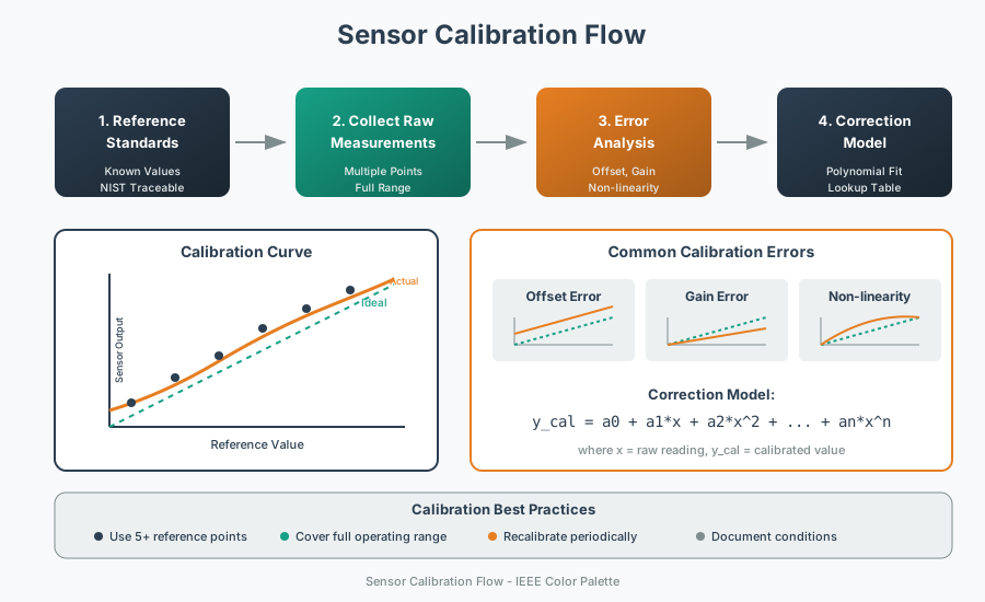
The electrical measurement comes before the temperature equation. In a common divider, the thermistor and a fixed resistor split the supply voltage; the ADC measures the middle node. With the fixed resistor tied to VCC and the thermistor tied to ground, R_thermistor = R_fixed * Vout / (Vin - Vout). Reversing the divider reverses the formula, so the first debug step is to confirm the schematic before blaming the math.
A practical calibration run records the raw ADC code, computed resistance, reference temperature, and model temperature in the same table. That table shows whether the error is random noise, a single-point offset, or a curve-fit problem. It also catches unit mistakes: the Beta equation uses kelvin, while lab notes and most datasheets report degrees Celsius.
Field tip: the Beta value itself is specified between two temperatures (e.g. 25/85 °C). Using a Beta calibrated for one range far outside it adds error, because Beta is only an approximation of the true curve.
Practitioner Knowledge Check
35.6 Under the Hood: When Beta Isn’t Enough
The Beta equation is a two-parameter fit, so it matches the true curve well near its calibration range and drifts away from it at the extremes. When you need accuracy across a wide span, you move to a richer model.
Steinhart-Hart equation
The three-term form 1/T = A + B·ln(R) + C·(ln R)^3 fits the thermistor curve across a wide range far better than Beta, typically to a small fraction of a degree once A, B, C are calibrated from three points.
RTDs curve too, just gently
Even a PT100 is not perfectly linear. High-accuracy work uses the Callendar–Van Dusen equation, adding second- and higher-order terms to the simple R0(1 + αT) approximation.
Sensitivity is not uniform
A thermistor is most sensitive near its nominal temperature and flattens far from it. Choosing the divider resistor near the thermistor's resistance at your target temperature keeps the reading in the sensitive region.
Self-heating shifts the reading
The current you push through the thermistor to read it dissipates power and warms the element slightly, biasing it upward. Keep the sense current low, especially in still air where heat cannot escape.
The coefficients also depend on the exact part, not just the sensor family. Two nominal 10 kΩ NTCs can share the same resistance at 25 °C yet diverge outside that point because their Beta values and tolerances differ. That is why production systems either buy a specified tolerance class, store per-device calibration constants, or calibrate the whole assembled channel rather than the bare component alone.
Model error and measurement error stack. Lead resistance is usually negligible for a 10 kΩ thermistor but can matter for low-resistance RTDs. ADC reference drift changes the computed divider ratio. Moisture or board leakage creates parallel resistance paths that look like a warmer thermistor. Long cables add pickup, so filtering can make the trace quieter without making the physics more correct.
The through-line is that a temperature reading is only as good as its model of the sensor's curve and its measurement chain. A cheap thermistor with a well-calibrated Steinhart-Hart fit can beat a nominally better sensor read through a careless linear approximation, while a high-grade RTD still fails if its excitation current, reference resistor, or lead compensation is ignored.
Under-the-Hood Knowledge Check
35.7 Release Checklist
Before relying on an analog temperature channel, confirm these points:
- The schematic orientation is documented so firmware converts ADC voltage into the correct resistance.
- The Beta value or Steinhart-Hart coefficients belong to the exact part and temperature range in use.
- Reference measurements include the operating range, not only room temperature.
- The ADC reference, fixed resistor tolerance, lead resistance, leakage paths, and filtering are included in the error budget.
- Sense current is low enough to avoid self-heating in still air or inside the enclosure.
- Validation records raw ADC code, computed resistance, reference temperature, model output, and residual error.
35.8 See Also
- Temperature Sensor Labs for DS18B20, DHT22, thermocouple, humidity, and lab workflows.
- Resistive Dividers and ADC Loading for divider-to-ADC measurement boundaries.
- Sensor Calibration Techniques for reference points, coefficient storage, and validation.
- Signal Conditioning for Sensors for analog filtering and ADC preparation.
35.9 Next
Return to Temperature Sensor Labs once the analog conversion model is bounded, then continue to Motion and Environmental Sensor Labs for the next lab family.