18 Calibration Taxonomy and Zero-Span
18.1 Start With the Measurement Story
A calibration problem is easier when the error has a name. Begin by asking whether the reading is shifted, stretched, curved, drifting, or hysteretic, because zero, span, and curve errors need different fixes.

Phoebe’s Why
This chapter’s “gain” is a calibration scale factor – a dimensionless multiplier near 1.0 that stretches a sensor’s raw reading to match a true reference span, like the \(1.0417\) worked out below. A radio’s “antenna gain” is a completely different physical quantity: a logarithmic ratio, in dBi, describing how much an antenna concentrates radiated power into a direction compared with a fictional isotropic radiator that spreads power evenly over the whole sphere. One is a linear correction applied to counts after the fact; the other is a geometric property of how energy leaves an antenna before the signal ever reaches a receiver. A review record that just writes “gain” without saying which one invites a very expensive mix-up.
The Derivation
Calibration span/gain (for contrast, from this chapter):
\[\text{gain}_{\text{cal}} = \frac{\text{true span}}{\text{measured span}}\]
Antenna gain relates a directional antenna’s solid angle \(\Omega\) to isotropic coverage:
\[G = \frac{4\pi}{\Omega}\]
Isotropic power density at distance \(d\), and with gain applied:
\[S_{iso} = \frac{P_t}{4\pi d^2} \qquad S = \frac{P_t G}{4\pi d^2}\]
Effective isotropic radiated power:
\[\mathrm{EIRP}_{dBm} = P_{t,dBm} + G_{dBi}\]
Worked Numbers: The Wireless Node Carrying This Sensor
- This chapter’s own gain, for contrast: \(\text{gain}_{\text{cal}} = 100/96 = 1.0417\) – a unitless correction, always near 1, applied to the sensor’s counts. It never appears in a link budget.
- Antenna gain on the node’s radio: catalog-typical 2.4 GHz sensor-node radio, \(P_t=0\) dBm \(=1\) mW, integrated chip antenna \(G=1.5\) dBi \(=10^{0.15}=1.41\times\). EIRP \(=0+1.5=1.50\) dBm \(=1.41\) mW.
- Swap to an external 5 dBi whip, same \(P_t=0\) dBm: \(G=10^{0.5}=3.16\times\), EIRP \(=5.00\) dBm \(=3.16\) mW.
- Range and coverage trade: range grows by \(\sqrt{3.16/1.41}=1.50\times\), while covered solid angle shrinks from \(1/1.41=70.8\%\) of the sphere to \(1/3.16=31.6\%\) – the same “trade coverage for range” pattern as the calibration span-gain example above, but on the RF side of the same node, and never to be added to the sensor’s own \(1.0417\).
18.2 Learning Objectives
After this page, you should be able to:
- Match offset, span, nonlinearity, drift, and hysteresis errors to the correction they can or cannot support.
- Run zero-and-span arithmetic from two reference readings without hiding the zero offset.
- Use residuals and holdout points to decide when a calibration model is overfit or out of range.
- Record traceability, expiry, and environmental evidence so calibration coefficients remain auditable.
18.3 After Calibration Techniques
Sensor Calibration Techniques introduces one-point, two-point, and multi-point calibration workflows with calculators and implementation examples. This page focuses on the decision logic behind those workflows: what kind of error is present, which correction is defensible, and what evidence should travel with the coefficients.
Use it before accepting a calibration record for a deployed IoT device, especially when the sensor has curvature, drift, temperature dependence, or a measurement claim that must survive review.
18.4 Calibration as a Toolbox
Calibration is often imagined as one action, but it is really a small toolbox of corrections, each aimed at a different kind of error. Match the tool to the error and the fix is clean; use the wrong tool and the error survives.
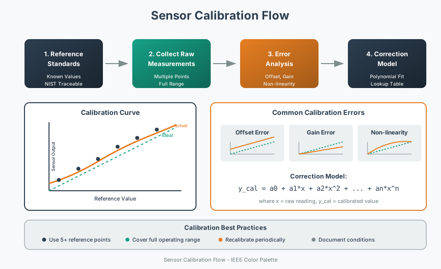
Three systematic errors have three matching corrections. A zero (offset) error is a constant shift, fixed by a one-point zero adjustment. A span (gain) error is a wrong scale, fixed by adding a second point. Nonlinearity is curvature the straight-line fit cannot follow, fixed by multiple points or a polynomial. A fourth problem, hysteresis, is path-dependent and cannot be removed by any of these — it has to be minimised in hardware and lived with as a spec.
In an IoT system, calibration is the boundary between a raw signal and a claim you can defend. A thermistor voltage, load-cell ADC count, or gas-sensor resistance is only an observation until it is tied to a reference standard with a date, environment, and method. That is why calibration records should name the reference instrument, the points used, the averaging window, and the final coefficients stored in firmware or cloud metadata.
The reference may be a traceable instrument or a physical condition that is stable enough for the claim: a NIST/NPL-traceable thermometer, a ruler or gauge block for a range sensor, an ice-water or boiling-water bath for temperature endpoints, or a 1 g orientation check for an accelerometer. The record should name the reference, its uncertainty, and the range it actually covered; otherwise calibration only maps one untrusted number onto another.
The number of reference points follows from the error you are trying to remove. One stable point can remove a zero shift, but it says nothing about slope. Two points define a straight line and therefore correct both zero and span across the calibrated range. Three or more points are evidence that the response bends; they can support a lookup table or low-order fit, but they also create a duty to validate at points that were not used to build the correction.
Intuition: zero correction slides the response, gain correction tilts it, linearity correction un-bends it. Knowing which of these your error is tells you exactly how many reference points you need.
Overview Knowledge Check
18.5 Practitioner: Zero-and-Span Correction
The everyday two-point calibration is best understood as two separate corrections: subtract the zero, then rescale by the gain.
Run the procedure like a measurement task, not a single button press. Let the sensor and reference settle, take several readings at each point, average them, and write down the conditions. Temperature, supply voltage, mounting stress, and warm-up time can all move the raw reading, so a coefficient produced from rushed data can look mathematically clean while still being wrong in the field.
Choose reference points that bracket the useful operating range. If a freezer monitor only needs -20°C to 10°C, a low reference near -20°C and a high reference near 10°C teach the firmware more than a distant boiling-water point. After fitting the line, reserve a third value as a holdout check. The corrected reading at that holdout should meet the product tolerance before the calibration is accepted.
| Error type | Character | Correction | Points needed |
|---|---|---|---|
| Zero / offset | Additive constant | Subtract measured zero | 1 |
| Span / gain | Multiplicative scale | Multiply by true span / measured span | 2 |
| Nonlinearity | Curvature | Multi-point table or polynomial | 3 or more |
| Hysteresis | Path-dependent | Not correctable by fit; minimise in hardware | — |
Worked example: zero-and-span on a 0–100 unit sensor
A checkout finds the sensor reads:
   2 units at a true 0    (zero error = +2)
  98 units at a true 100

  measured span = 98 - 2 = 96
  gain          = true span / measured span = 100 / 96 = 1.0417

  corrected = gain × (raw - zero)
            = 1.0417 × (raw - 2)

Check at raw = 98:  1.0417 × (98 - 2) = 1.0417 × 96 = 100  ✓
Check at raw = 2:   1.0417 × (2  - 2) = 0                  ✓
Splitting the fix into "remove the zero, then scale the span" makes it obvious why you need exactly two points: one to find the zero, a second to find the gain.
For deployment, store more than just the two numbers. A useful record includes the raw low/high readings, the true reference values, the computed zero and gain, the technician or fixture ID, and the firmware version that applied the calculation. If a later batch starts failing validation, those records let you separate a bad sensor lot from a software regression or a drifting reference standard.
Practitioner Knowledge Check
18.6 Polynomial Calibration Risks
When curvature remains after zero-and-span, you reach for more points — but more is not always better, and no calibration lasts forever. The engineering problem is not to make a pretty curve through the calibration points; it is to reduce residual error across the range where the sensor will actually be trusted.
Start by plotting residuals: corrected value minus reference value at every calibration and validation point. If the residuals are randomly small, the model is probably adequate. If they arc upward or downward, the model is missing curvature. If they are small at the fit points but large between them, the fit is probably too flexible. A simple lookup table with interpolation is often safer than a high-order polynomial because its behavior between adjacent reference points is easier to inspect.
Linearity is also conditional. Temperature, vibration, acoustic noise, humidity, supply voltage, mounting stress, and bandwidth can move the residual curve after the neat bench plot is finished. A sensor may look linear during slow sweeps but distort rapidly changing inputs because the transducer, package, filter, or ADC front end adds amplitude lag, phase shift, or harmonics. If those error harmonics fall into the same band as the signal of interest, a polynomial fitted from DC reference points will not rescue the measurement. Dynamic nonlinearity needs a time-domain or frequency-sweep check, with bandwidth and response-time limits recorded beside the calibration curve.
Polynomial linearization
Fit corrected = a0 + a1·x + a2·x^2 + ... from several reference points to model the curve. A second- or third-order fit usually captures smooth sensor curvature well.
Overfitting and extrapolation
Too high an order chases measurement noise instead of the true curve and can swing wildly just outside the calibrated range. Use the lowest order that meets the spec, and never trust it beyond the points.
Look-up tables as an alternative
A multi-point table with interpolation avoids overfitting entirely and behaves predictably, at the cost of storing the points. It is often the robust choice for awkward, non-polynomial curves.
Calibration has an expiry
Sensors drift with time and temperature (quoted as %FS per year, ppm per °C). The recalibration interval is set by how much drift you can tolerate; a temperature reading lets firmware compensate the tempco between calibrations.
Drift turns calibration into a lifecycle decision. Suppose a 0–100 unit sensor is allowed 0.5 units of total measurement error and its datasheet drift is 0.2% of full scale per year, or 0.2 units/year. If the initial calibration already consumes 0.1 units of the budget, only 0.4 units remain for drift. A simple limit gives 0.4 / 0.2 = 2 years before the budget is exhausted; a maintenance plan might set the recalibration interval to 12 or 18 months to leave margin for harsh conditions and reference uncertainty.
Two final disciplines separate a calibration you can defend from one you cannot. Traceability: the fit is only as good as the reference standard, so record what you calibrated against and when, including the reference accuracy. Honesty about hysteresis: it is path-dependent, so no offset, gain, or polynomial removes it — it must be designed out, tested in both directions, and then stated as a residual uncertainty. Range discipline matters too: outside the lowest and highest reference points, the correction is an extrapolation, not a calibration.
Under-the-Hood Knowledge Check
18.7 Release Checklist
Before accepting calibration coefficients, confirm these points:
- The reference standards bracket the operating range that the device will actually use.
- Offset, gain, nonlinearity, drift, and hysteresis have been separated instead of folded into one unexplained number.
- At least one holdout point not used in the fit validates the corrected reading against the product tolerance.
- The stored record includes raw readings, true references, environmental conditions, reference instrument ID, firmware version, and calibration date.
- The recalibration interval follows the drift budget rather than a generic calendar guess.
- Readings outside the lowest and highest reference points are labelled as extrapolations, not calibrated values.
18.8 See Also
- Sensor Calibration Techniques for the main workflow, calculators, and coefficient-storage examples.
- Sensor Calibration Lab for hands-on calibration and validation practice.
- Span Validation and Release Evidence for range guards, residuals, release labels, and validation evidence.
- Accuracy, Precision, Drift, and Hysteresis for reporting residual uncertainty after calibration.
18.9 Next
Return to Sensor Calibration Techniques once the error model is clear, then continue to Sensor Calibration Lab to practice validation with a full sensor workflow.