31 Braitenberg Transfer Tuning
31.1 Start With the Measurement Story
A reactive rule only works if the sensor curve and motor response are understood. Begin with the transfer story: how raw light becomes resistance, how that becomes speed, and where saturation or lag breaks the reflex.
31.2 Learning Objectives
After this page, you should be able to:
- Explain why a sensor transfer function can change a Braitenberg vehicle’s apparent behavior.
- Predict where LDR compression, saturation, and response lag will cause steering errors.
- Tune divider, dead-band, scaling, and motor mapping choices from bench evidence.
- Implement and test multi-mode reactive behavior before escalating to AI/ML.
31.3 After Braitenberg Basics
Braitenberg Vehicles: Sensing to Action explains how topology and polarity create reactive behavior. This page tests the physical measurement chain behind those rules: a simple mapping only stays simple if the sensor curve, conditioning circuit, motor scaling, and timing lag are known.
31.4 Transfer Function as Behavior
A Braitenberg vehicle wires a sensor almost directly to a motor, so the vehicle’s personality is decided by one thing: the sensor’s transfer function — the rule that maps the physical stimulus (say, light level) to the output signal (a voltage that drives the wheel). Change the shape of that curve and you change how the vehicle acts.
This is why “more light means more signal” is not enough to predict behaviour. A light sensor that responds steeply in dim conditions but barely at all in bright ones will make a vehicle lunge toward a distant lamp yet crawl once it is close. The shape of the curve — where it is steep, where it flattens — is the design.
For a light-following robot, the curve is part of the steering loop. If the left light sensor climbs from 10 to 100 lux while the right sensor stays near 10 lux, the left-side signal changes strongly and the vehicle turns. If both sensors are already near saturation at 900 and 1000 lux, the signal difference may be tiny even though the physical light difference is real. The vehicle then appears indecisive near the lamp.
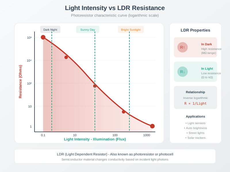
A useful bench check is to sweep the sensor with a desk lamp before connecting the motors. Record output at several distances, then ask where the curve is steep enough to steer and where it is flat enough to hide differences. That simple plot predicts most of the vehicle’s “personality” before the chassis moves.
Intuition: the transfer function is the vehicle’s reflexes. A gentle, gradual curve gives calm, proportional reactions; a steep or saturating curve gives twitchy, all-or-nothing ones. The same wiring feels completely different behind a different sensor curve.
Overview Knowledge Check
31.5 Photoresistor Compression Loop
Sensitivity is the local slope of the transfer function, and for many real sensors that slope changes along the curve. A photoresistor (LDR/CdS cell) is a classic example: its resistance follows a power law in illuminance, so it is compressive.
Sensitivity = d(output) / d(stimulus)   (the local slope, not a constant)
Photoresistor: R = R_ref × (E / E_ref)^(-γ)
  E = illuminance,  γ ≈ 0.6 to 0.9 for a CdS cell (a compressive, log-like law)
Worked example: equal light ratios, shrinking resistance steps
LDR: R = 10 kΩ at 10 lux, γ = 0.7

  At 100 lux (10x brighter):
R = 10k × (100/10)^-0.7 = 10k × 10^-0.7 = 10k × 0.20 = 2.0 kΩ
  At 1000 lux (another 10x):
R = 10k × (1000/10)^-0.7 = 10k × 100^-0.7 = 10k × 0.04 = 0.4 kΩ

Each 10x jump in light multiplies R by the same 0.20,
so the resistance CHANGE shrinks: 8 kΩ then 1.6 kΩ.
The sensor is far more responsive in dim light than bright.
For the vehicle, that compressive curve means strong reactions to a faint, distant light and muted reactions once the light is close and bright — behaviour that comes entirely from the sensor’s curve, not from any code.
Now put that LDR into a voltage divider with a 10 kΩ fixed resistor to ground and a 3.3 V supply. With the LDR as the top resistor, Vout = 3.3 × 10k / (Rldr + 10k). At 10 lux, Rldr = 10 kΩ, so Vout = 1.65 V. At 100 lux, Rldr = 2 kΩ, so Vout = 2.75 V. At 1000 lux, Rldr = 0.4 kΩ, so Vout = 3.17 V.
The first 10x light increase moves the signal by about 1.10 V; the next 10x increase moves it by only 0.42 V. A microcontroller or motor driver sees those voltages, not the lux directly. So the effective vehicle rule is not “turn proportional to light”; it is “turn proportional to the conditioned voltage curve.”
Practitioner Knowledge Check

Phoebe’s Why
The LDR’s power law is not an arbitrary curve fit – it falls out of what light actually does inside the cell. Photons with enough energy knock electrons loose, creating extra charge carriers at a rate set by the light level. Those carriers do not pile up forever; they recombine and disappear, and the shape of that recombination is what decides the exponent this chapter calls \(\gamma\). If every extra carrier disappears at a rate proportional to its own population (the simplest case, like a fixed number of trap sites each catching one carrier), the steady-state carrier count rises exactly as fast as the light does, and resistance would fall as a clean inverse of illuminance. If instead carriers mostly vanish by finding each other and recombining in pairs, doubling the light only raises the steady-state population by the square root of two, because each new carrier now has more partners to recombine with. Real CdS cells sit between those two limits, which is exactly why this chapter’s own \(\gamma\approx0.6\) to \(0.9\) is a compromise value, not a round number.
The Derivation
Steady state balances photon-driven generation \(G\) (proportional to illuminance \(E\)) against recombination:
\[\frac{dn}{dt} = G - R(n) = 0\]
Trap-limited (monomolecular) recombination gives a linear response:
\[R(n)=\frac{n}{\tau_0}\ \Rightarrow\ n = G\tau_0 \propto E^{1} \quad(\gamma = 1)\]
Free-carrier (bimolecular) recombination gives a square-root response:
\[R(n)=\beta n^{2}\ \Rightarrow\ n = \sqrt{G/\beta} \propto E^{0.5} \quad(\gamma = 0.5)\]
Since conductance \(\propto n\), resistance is the inverse, \(R \propto E^{-\gamma}\) with \(0.5 \le \gamma \le 1\) – the chapter’s own power law, now with a physical floor and ceiling instead of an assumed exponent.
Worked Numbers: This Chapter’s Own 10 kΩ, γ = 0.7 Cell
- Where 0.7 sits: \(0.5 \le 0.7 \le 1.0\) – squarely between the bimolecular floor and the monomolecular ceiling, consistent with a cell whose recombination is a mix of both mechanisms rather than either idealized case.
- Self-check against this chapter’s own numbers: \(R(100\ \text{lux}) = 10\,\text{k}\Omega\times(100/10)^{-0.7} = 10\times10^{-0.7} = 1.995\ \text{k}\Omega \approx 2.0\ \text{k}\Omega\), and \(R(1000\ \text{lux}) = 10\,\text{k}\Omega\times100^{-0.7} = 0.398\ \text{k}\Omega \approx 0.4\ \text{k}\Omega\) – both match this chapter’s stated 2 kΩ and 0.4 kΩ exactly.
- Divider voltage, recomputed to more places: with the chapter’s own 10 kΩ fixed resistor and 3.3 V rail, \(V_{out}=1.6500\) V at 10 lux, \(2.7511\) V at 100 lux, \(3.1737\) V at 1000 lux – steps of \(1.1011\) V then \(0.4226\) V, matching this chapter’s “about 1.10 V, then only 0.42 V” to four figures.
- What a different \(\gamma\) would have done: at the monomolecular ceiling \(\gamma=1.0\), the same two decades of light would swing \(R\) from 10 kΩ all the way to 0.1 kΩ (a 100× span instead of 25×) – a steeper, even more compressive curve, and a twitchier vehicle than this chapter’s actual \(\gamma=0.7\) cell produces.
31.6 Curve Shaping and Photoresistor Memory
Once you see behaviour as a consequence of the transfer function, you can engineer it — and you can also spot where a real sensor will betray you.
The full controller is the product of three curves: physical stimulus to sensor output, sensor output to conditioned voltage, and conditioned voltage to actuator command. A different divider resistor, ADC reference, dead band, PWM mapping, or motor driver gain changes the behaviour even when the wiring diagram stays the same. That is why a bench plot of voltage versus lux is more useful than a single "LDR sensitivity" number.
Photoresistors add one more complication: memory. CdS cells can take tens or hundreds of milliseconds to brighten and longer to recover after bright exposure. A fast robot may therefore steer using yesterday's light reading for part of a turn. In a Braitenberg loop, that lag is feedback delay; too much delay causes oscillation, hunting, or overshoot around the stimulus.
Linear, compressive, saturating
A linear curve gives proportional reactions; a compressive (log-like) curve stays responsive across a huge range but dulls when strong; a saturating curve flattens above a level, so the vehicle cannot tell a bright light from a brighter one.
Sensitivity dies at saturation
Where the curve flattens, the local slope approaches zero, so 900 and 1000 lux produce nearly the same signal. Near a lamp a saturating sensor makes the vehicle blind to further increases.
You can reshape it with conditioning
The divider resistor, and any log or linearising amplifier, changes the overall stimulus-to-voltage curve. Sensor plus conditioning equals the effective transfer function, which is the real behaviour lever.
The CdS memory effect
Photoresistors respond slowly (tens of milliseconds to seconds) and show light-history hysteresis: the same illuminance can read differently depending on prior exposure. A fast-moving vehicle can lag and behave inconsistently because of it.
The lesson generalises well beyond toy robots: whenever a sensor drives an action with little processing in between, the transfer function is the controller. Choosing or shaping that curve — and knowing where it saturates or lags — is how you get the behaviour you intend rather than the one the raw sensor happens to give. A practical validation run should therefore log raw lux or resistance, conditioned voltage, PWM command, and observed turn direction at several distances from the lamp.
Under-the-Hood Knowledge Check
31.7 Beginner Build: Light-Following Robot
Goal: Build Vehicle 2b that chases a flashlight.
Components:
- ESP32 + L298N motor driver
- 2× LDR photoresistors (left/right sensors)
- 2× DC motors + wheels
- 9V battery
Wiring:
Left LDR  → ADC pin 34 → Right motor (cross-wired)
Right LDR → ADC pin 35 → Left motor (cross-wired)
More light = faster motor (excitatory)
Expected behavior: Robot turns toward flashlight and drives into it
31.8 Temperature-Seeking Heater
Goal: Build a mobile heater that moves toward warm areas and stays there (for temperature monitoring or co-locating with existing heat sources).
Components:
- 2x thermistors (left/right temperature sensors)
- 2x DC motors
- Temperature logger / display
Wiring topology:
- Same-side inhibitory (love behavior)
- Warm side (high temp reading) inhibits same-side motor more, slowing it -> turns toward warmth
- As it reaches the warm zone, both sensors read high, both motors slow -> stops near the heat source
Why this works: Same-side inhibitory means motor = base_speed - sensor * gain. High stimulus (warmth) produces high inhibition, slowing the motor on that side. The opposite motor runs faster, turning the vehicle toward the warm area. Near the source, both sensors read high, both motors slow, and the vehicle stops – classic “love” behavior.
Real application: A mobile sensor platform that autonomously navigates to warm zones for thermal monitoring, or a robot that finds and stays near a charging station emitting heat.
31.9 Multi-Behavior State Machine
Goal: Robot switches between fear/aggression/love modes using a button.
Modes:
- Fear mode (same-side excitatory): Runs from light
- Aggression mode (cross-wired excitatory): Attacks light
- Love mode (same-side inhibitory): Approaches and stops near light
Challenge: Implement smooth transitions between modes, add LED indicators for current mode
Bonus: Add a fourth mode: “Explorer” (cross-wired inhibitory) for obstacle avoidance (Roomba-like)
31.10 Reactive Design Rule Practice
31.11 Concept Relationships
| Core Concept | Related Concepts | Why It Matters |
|---|---|---|
| Cross-Wired vs Same-Side | Approach vs Avoidance | Determines direction of response |
| Excitatory vs Inhibitory | Speed Up vs Slow Down | Determines intensity of response |
| Emergent Behavior | Simple Rules, Complex Outcomes | Intelligence appears without programming it |
| Reactive Control | No Memory, Fast Response | Simpler than AI, often sufficient |
Common Pitfalls
An excitatory connection increases motor speed when the sensor signal increases; an inhibitory connection decreases motor speed. Swapping these causes vehicles to move opposite to intended — approach instead of avoid. Always simulate the behavior on paper before wiring physical motors.
If the sensor output range drives motor speed directly without scaling, the motor may always run at maximum or minimum speed with little intermediate behavior. Add a scaling function between the sensor output and the motor driver to use the full behavioral range.
Physical motors have inertia and time constants (50-500 ms) that lag behind rapidly changing sensor inputs, causing jittery oscillatory motion. Add a low-pass filter to the sensor input or a ramp-rate limit on the motor command to achieve smooth behavior.
A vehicle controlled by a single light sensor fails unpredictably when walls, reflections, or shadows create contradictory stimuli. Add a second sensor type (proximity, IR distance) to provide context and enable more situation-aware behaviors.
31.12 Release Checklist
Before accepting a Braitenberg-style reactive controller, capture this evidence:
- Sensor output measured across the expected stimulus range, including saturation points.
- Conditioned voltage or ADC count plotted against physical stimulus, not just raw sensor resistance.
- Motor command scaling, dead band, and ramp limits chosen from bench tests.
- Delay or hysteresis measured for sensors such as LDRs before fast-motion tests.
- Mode-switching behavior verified for every wiring/polarity combination.
- A documented decision that reactive control is sufficient, or a trigger for escalating to AI/ML.
31.13 See Also
- Braitenberg Vehicles: Sensing to Action - core wiring and behavior model
- Sensor Signal Conditioning - shaping analog signals before control
- Common Sensor Mistakes - broader sensing failure patterns
31.14 What’s Next
Return to Braitenberg Vehicles for the main module path, or continue to Infrastructure Sensing for reactive systems built from existing signals.