16 Sampling and Anti-Alias Limits
Nyquist Limits Before Sensor Filtering
sensor sampling, Nyquist, aliasing, anti-alias filter, ADC, oversampling
16.1 Start With the Measurement Story
A waveform sampled too slowly can tell a confident lie. The design story begins with how fast the physical signal can change, what frequencies must be kept, and what filtering is needed before the ADC samples it.

Phoebe’s Why
Quantization is a rounding error, and if it lands anywhere in one code step with equal probability, its RMS size is a fixed fraction of that step, \(q/\sqrt{12}\). Average several independent readings and that RMS error – being random and uncorrelated between readings – shrinks like the square root of the count, not the count itself. That is the real reason this chapter’s own four-sample average earns only a 2x cleanup: \(\sqrt{4}=2\). It is also exactly why oversampling cannot rescue an alias: a coherent 90 Hz tone that has already folded to 10 Hz is not random noise scattered across readings, it is the same wrong value repeated every time, so averaging preserves it instead of cancelling it.
The Derivation
Quantization step and its RMS noise-floor equivalent:
\[q = \frac{V_{ref}}{2^N}, \qquad e_{rms}(1) = \frac{q}{\sqrt{12}}\]
Averaging \(M\) independent readings shrinks that RMS error by the square root of the count:
\[e_{rms}(M) = \frac{e_{rms}(1)}{\sqrt{M}}\]
which converts to a decibel gain and an equivalent number of extra effective bits:
\[\mathrm{SNR\ gain} = 10\log_{10}(M)\ \text{dB}, \qquad \text{extra bits} = \frac{10\log_{10}(M)}{6.02}\]
Worked Numbers: This Chapter’s Own Averaging Claim
- \(M=4\) (this chapter’s own example): \(\mathrm{SNR\ gain}=10\log_{10}(4)=6.02\) dB, extra bits \(=6.02/6.02=1.00\) – matching the chapter’s own “about 2:1, roughly one extra effective bit” exactly
- \(M=16\): \(\mathrm{SNR\ gain}=10\log_{10}(16)=12.0\) dB, extra bits \(=2.00\) – confirms the \(1/\sqrt{M}\) pattern: quadrupling the sample count again, not doubling it, is what buys the next full bit
- What averaging cannot touch: this chapter’s own 90 Hz interferer aliased to 10 Hz is a fixed, repeatable value at every sample, not an independent random error, so no amount of \(M\) averages it down – the \(1/\sqrt{M}\) benefit above applies only to genuinely random quantization and circuit noise, never to an alias
16.2 Learning Objectives
After this page, you should be able to:
- Explain why sampling happens before firmware filtering and calibration.
- Use the Nyquist rule to identify sample rates that can alias sensor signals.
- Calculate where an out-of-band frequency appears after sampling.
- Place analog anti-alias filtering before the ADC and digital filtering after it.
- Decide when oversampling helps noise performance without pretending to fix aliasing.
16.3 After Data Processing
Sensor Data Processing teaches moving averages, median filters, calibration equations, validation rules, and persistence of calibration coefficients. Those techniques assume the ADC already captured the physical signal correctly. This page checks the boundary before that assumption: the analog sensor path, sample rate, and anti-alias filter determine whether the data is real signal or a believable artifact.
A practical deployment treats acquisition and processing as one contract. If the logger samples too slowly, a vibration, motor-drive ripple, or power-line component can fold into the operating band and survive every later average, calibration, dashboard, and alert rule. Use this page before tuning firmware filters when a signal changes after a sample-rate change, appears at an implausible frequency, or arrives from an analog path without a documented bandwidth limit.
16.4 Snapshots of a Continuous World
The physical world is continuous, but a data pipeline sees only snapshots: the ADC captures the signal at a fixed sample rate fs and throws away everything in between. If the signal changes slowly compared with how often you sample, the snapshots faithfully trace it. If it changes quickly, the snapshots can lie.
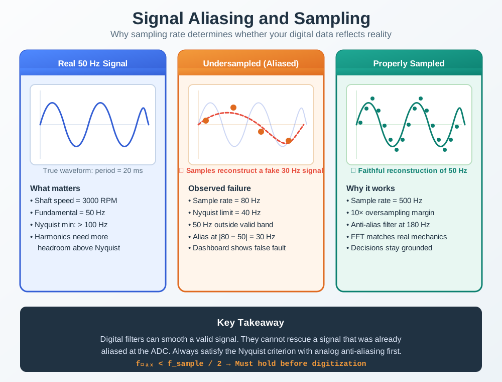
When a signal contains frequencies faster than half the sample rate, those fast components reappear disguised as slow ones. This is aliasing, and it is the single most damaging mistake in sensor data acquisition, because the result looks like perfectly plausible data. The guard against it is the Nyquist rule: sample at more than twice the highest frequency present in the signal.
Intuition: a fast-spinning wheel filmed at a slow frame rate can appear to turn backwards or stand still. The camera is under-sampling the motion. An ADC that samples too slowly does exactly the same thing to a sensor signal.
As a concrete acquisition check, imagine an accelerometer on a small pump. The mechanical signal of interest is shaft imbalance around 12 Hz, but the motor drive injects a 38 Hz ripple onto the analog line. If the logger samples at 50 samples/s, Nyquist is 25 Hz, so the 38 Hz ripple cannot be represented honestly. It folds to |38 - 50 x round(38/50)| = 12 Hz, exactly where the real imbalance feature lives. The trend plot now shows a believable 12 Hz vibration even if the shaft is healthy. The fix is not a smarter dashboard; it is sampling and filtering so the 38 Hz component cannot enter the ADC path.
A quick field test is to repeat the capture at a different sample rate. A real 12 Hz vibration stays at 12 Hz when you move from 50 SPS to 80 SPS. The aliased 38 Hz interference moves from 12 Hz at 50 SPS to |38 - 80 x round(38/80)| = 38 Hz, safely below the new 40 Hz Nyquist limit. If the apparent feature moves when the sample rate changes, suspect aliasing before diagnosing the machine.
Overview Knowledge Check
16.5 Predicting Frequency Aliases
When a component at frequency f is sampled at fs, it appears at an aliased frequency:
f_alias = | f - fs × round(f / fs) |     (valid up to fs/2)
Nyquist frequency = fs / 2
Worked example: machine vibration on a 50 SPS logger
Sample rate fs = 50 samples/s  ->  Nyquist = 25 Hz

A 30 Hz vibration component (above 25 Hz) aliases:
  round(30/50) = round(0.6) = 1
  f_alias = |30 - 50 × 1| = 20 Hz

A 55 Hz component aliases:
  round(55/50) = round(1.1) = 1
  f_alias = |55 - 50 × 1| = 5 Hz
The 30 Hz vibration shows up in your logs as a phantom 20 Hz tone, and 55 Hz noise appears as a slow 5 Hz wander. Neither is real, yet both look like legitimate signal. No amount of downstream processing can tell them apart from a true 20 Hz or 5 Hz signal.
Turn that into a design rule before deployment. If the fastest useful vibration feature is 20 Hz, sampling at 50 SPS gives a 25 Hz Nyquist limit with almost no room for a real analog filter to roll off. A safer design might sample at 200 SPS, place an analog low-pass near 40 Hz to suppress higher-frequency electrical noise, then apply a digital low-pass and decimate to 50 SPS for storage. The stored data rate is still small, but the analog front end had enough bandwidth margin to prevent false low-frequency content.
The fix goes before the ADC: an analog anti-alias low-pass filter that attenuates everything above fs/2 before the signal is sampled. A moving average or other digital filter applied after sampling smooths noise but cannot remove an alias, because the fast component is already gone — folded permanently into the low band.
Practitioner Knowledge Check
16.6 Aliasing and Oversampling Limits
Once a fast component has folded into the low band, the sampled sequence is identical to what a genuine low-frequency signal would have produced. There is no information left that distinguishes them, so no algorithm can separate them after the fact. That is why the anti-alias filter has to be analog and has to sit before the sampler.
The optional mathematics panel below works only with numbers already used in this chapter: the 12 Hz pump feature, the 38 Hz ripple, the 50 SPS and 80 SPS field test, the 200 SPS safer capture, the 40 Hz analog cutoff, and the four-sample oversampling example. It shows the arithmetic so the sampling decision can be checked rather than trusted.
Real filters are not brick walls
An analog low-pass filter rolls off gradually, not vertically at fs/2. So designers sample somewhat above twice the signal band (oversample) and set the filter cutoff below fs/2 with margin, leaving room for the roll-off.
Oversampling then decimating
Sampling far faster than needed, filtering digitally, then downsampling relaxes the analog filter and can trade excess rate for extra effective resolution — the principle behind sigma-delta ADCs.
Smoothing is not anti-aliasing
A moving average is a digital low-pass that reduces noise within the captured band. It runs after sampling, so it cannot recover or remove an alias that entered at sample time.
Band-limit at the source
The safest designs limit the signal bandwidth in the analog domain (sensor + filter) so that nothing above fs/2 ever reaches the ADC, rather than hoping the environment stays quiet.
Oversampling also improves noise handling, but only under the right assumptions. Averaging four independent samples can improve signal-to-noise ratio by about 2:1, roughly one extra effective bit, because random noise partially cancels. That benefit does not apply to a coherent 90 Hz interferer that has already aliased to 10 Hz; every decimated record will faithfully preserve the false tone. In practice, use oversampling to relax analog-filter steepness and reduce broadband noise, while still ensuring the analog input is band-limited before the first sample is taken.
The order of operations is the whole lesson: band-limit in analog, then sample. Reverse that order and the data is corrupted before your firmware ever touches it.
Under-the-Hood Knowledge Check
16.7 Release Checklist
Before relying on a processed sensor stream, confirm the acquisition chain has evidence for each item:
- The highest expected signal frequency and likely interference frequencies are documented.
- The chosen sample rate leaves margin above twice the highest frequency that can reach the ADC.
- The analog anti-alias filter cutoff is below Nyquist and before the ADC input.
- A sample-rate change test distinguishes real features from movable aliases.
- Digital filtering is used only after acquisition has prevented irreversible aliasing.
16.8 See Also
- Sensor Data Processing for filtering, calibration, validation, and persistence patterns.
- Signal Conditioning for analog front-end design before ADC conversion.
- Signal Processing for IoT Sensors for additional filtering and transform tools.
- Multi-Sensor Data Fusion for combining already trustworthy sensor readings.
16.9 Next
Return to Sensor Data Processing when the acquisition boundary is verified, then choose the digital filter and calibration method that matches the captured signal.