8 Sensor Selection Matrices
8.1 Start With the Measurement Story
A fit matrix turns a vague sensor debate into visible evidence. Each row asks whether the candidate survives the real constraints: measurement range, noise, power, mounting, calibration effort, cost, and failure behavior.
8.2 Learning Objectives
After this page, you should be able to:
- Treat sensor selection as a gated fit problem across range, resolution, accuracy, and response time.
- Record candidate evidence in a fit matrix so rejected sensors do not reappear with unresolved gaps.
- Explain range-resolution, response-noise, and headline-accuracy trade-offs in sensor comparisons.
- Identify when changes to the measurement chain require a sensor choice to be revalidated.
8.3 After Sensor Selection
Choosing the Right Sensor introduces requirements, shortlists, weighted scoring, datasheet checks, and production constraints. This page separates the deeper boundary material: how to prove that a candidate really fits the measurement problem before price, interface, and availability decide the winner.
Use it when a shortlist looks plausible but the decision still needs auditable evidence about measurement gates, unresolved assumptions, error budgets, and retest triggers.
8.4 Four-Axis Sensor Matching
Picking a sensor is not about finding the "best" one; it is about finding one whose specifications bracket your requirement on four axes at the same time. Win on one axis and fail another, and it is the wrong sensor.
Start by writing the measurement decision in plain language: what condition must the system observe, what action depends on it, and what error would change that action? That wording stops the selection process from drifting toward feature shopping. A greenhouse logger, safety alarm, predictive-maintenance node, and classroom demo may all measure temperature, but they tolerate different errors, response delays, calibration burdens, enclosure constraints, and maintenance costs.
- Range — can it span the full set of values you will see, with margin?
- Resolution — can it see the smallest change that matters to you?
- Accuracy — is it close enough to the true value for your tolerance?
- Response time / bandwidth — is it fast enough for how quickly the signal moves?
Only after those measurement gates pass should interface, power, package, availability, and price decide the winner. Those later filters matter, but they cannot rescue a candidate that cannot observe the required physical condition with enough trust.
Also separate must-have requirements from preferences before scoring. A must-have, such as an outdoor probe, certified safety rating, or required interface voltage, is a gate. A preference, such as lower unit price or extra humidity data, can be weighted after all gates pass. Mixing those categories is how a spreadsheet accidentally ranks a cheap but unusable sensor above a deployable one.
Intuition: think of it as four gates in a row. A candidate must pass every gate. A spectacular score at one gate never buys forgiveness at another — the weakest axis decides.
Overview Knowledge Check
8.5 Which Sensor Decision Example
Turn the requirement into concrete numbers, then test each candidate against every gate.
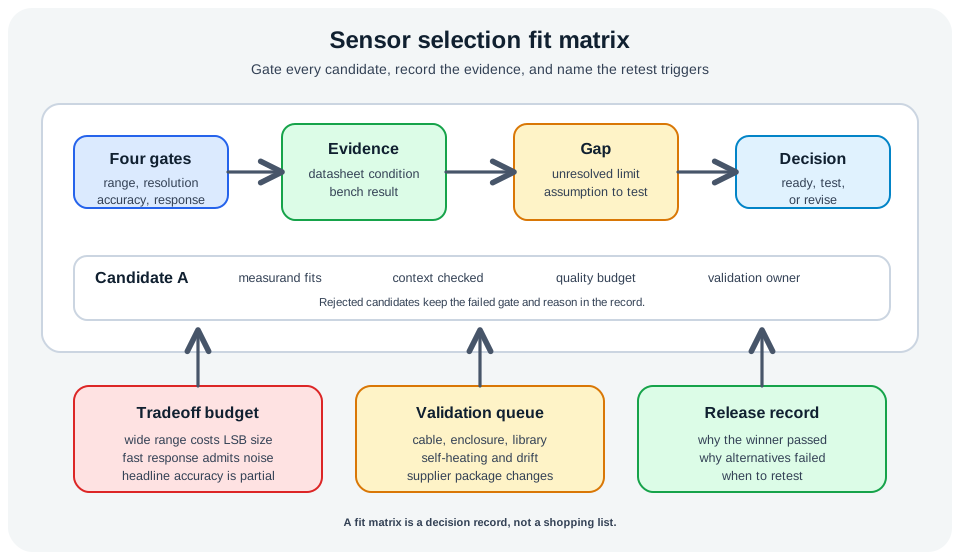
A useful shortlist records both pass and fail evidence. For each candidate, keep the exact datasheet value, the condition attached to that value, and the reason a failure matters. If a sensor fails waterproofing, say whether that is because the bare package lacks protection, because the cable gland is weaker than the probe, or because the supplier does not specify ingress protection. That level of detail prevents a rejected candidate from reappearing later as a "cheap alternative" with the same unresolved gap.
Requirement: a refrigerator monitor
Measure −20 to +10 °C, resolve 0.5 °C changes, accuracy within ±1 °C, temperature moves slowly (over minutes).
| Candidate | Range | Resolution | Accuracy | Verdict |
|---|---|---|---|---|
| A: digital IC sensor | −40 to +125 °C ✓ | 0.0625 °C ✓ | ±0.5 °C ✓ | Fits all four gates |
| B: bare thermocouple | very wide ✓ | fine ✓ | ±2 °C without careful cold-junction ✗ | Fails accuracy |
| C: analog sensor on 8-bit ADC | ok ✓ | LSB too coarse over range ✗ | — | Fails resolution |
Only candidate A passes every gate. Note that response time is a non-issue here because the fridge changes slowly — but for a fast process, a slow sensor would fail the fourth gate even if it aced the first three.
The same record should include what you still have to test. A candidate can pass on paper and still need a bench check for cable length, self-heating, condensation, library timing, pull-up values, or enclosure placement. Treat the shortlist as a decision record with a validation queue, not as a shopping list.
When two candidates both pass, prefer the one with fewer unresolved assumptions, not just the higher feature count. A simple digital temperature IC with a clear library, stable package, and known calibration path can beat a multi-sensor module if the extra signals are not used by the application decision.
Practitioner Knowledge Check
8.6 Sensor Tradeoff Axes
The four gates are not independent knobs you can max out separately. Several of them pull against each other, so selection is really about balancing an error budget.
That error budget has layers. The sensor element contributes offset, gain error, noise, hysteresis, drift, and cross-sensitivity. The interface can add ADC quantization, reference-voltage error, bus timing limits, pull-up loading, or conversion latency. The installation adds mounting stress, heat from nearby electronics, airflow blockage, vibration, condensation, dirt, and cable effects. A good selection compares the whole evidence path, not just the sensor chip.
The same layering applies to time. A fast sensor can still produce stale evidence if the firmware wakes slowly, the bus is congested, the filter window is long, or the radio batches reports. A slow sensor can be acceptable when the physical process changes over minutes or hours. Selection should therefore compare response time, sampling interval, processing delay, and reporting interval against the actual decision deadline.
Power has the same system-level trap. A datasheet may advertise a very low sensor sleep current, but the selected mode can require a long warm-up, repeated bus transactions, or a high-current reference circuit that keeps the controller awake. Conversely, a sensor with a slightly higher active current can still win if it converts quickly, lets the MCU sleep sooner, and avoids calibration visits. Under the hood, compare total energy, total error, and total maintenance effort, not isolated headline numbers. The best choice is the one whose tradeoffs stay inside the whole system budget.
Range vs resolution
For a fixed bit depth, LSB = range / 2^N, so a wider range means a coarser step. Choosing a range far larger than you need quietly throws away resolution; match the range to the real span plus modest margin.
Response time vs noise
Faster response means wider bandwidth, and wider bandwidth admits more noise. Slowing down or averaging quietens the reading but adds lag. Pick the slowest response that still tracks the signal's real dynamics.
Headline accuracy is not the whole error
The real budget adds initial accuracy, drift over the recalibration interval, temperature effects, and noise. Independent random parts combine in quadrature; systematic parts add. Check the total against your tolerance, not just the datasheet's best number.
The weakest axis dominates
Over-specifying one axis cannot rescue a failure on another: 24-bit resolution does not fix ±2 °C accuracy, and huge range does not fix a coarse LSB over that range. The worst gate sets the result.
So a disciplined selection writes the requirement as four numbers, builds a small error budget for accuracy over the deployment lifetime, and confirms the response time suits the signal's dynamics (which also sets the sample rate, back to Nyquist). Interface, power, and environment then filter what remains — but a sensor that fails any of the four measurement gates never makes it that far.
Production selection also includes the negative evidence. If a high-accuracy part fails because the factory calibration expires before the maintenance interval, the record should say that. If a low-power part fails because its conversion time forces a longer MCU wake window, record the system-level power cost rather than only the sensor current. Under the hood, the chosen sensor is the one whose remaining risks are explicit, tested, and acceptable.
Finally, selection is reversible only when the record preserves why alternatives lost. Supplier changes, board revisions, and firmware updates often reopen the choice. If the old record names the failed gates and validation evidence, the team can re-evaluate quickly without repeating the whole search from memory.
That retest discipline matters because the winning sensor is part of a larger measurement chain. Changing the ADC reference, enclosure material, cable length, firmware filter, sampling interval, calibration interval, or supplier package can invalidate an earlier pass. The selection record should name those dependencies so future maintenance work knows when a sensor is still acceptable and when the evidence has expired.
Under-the-Hood Knowledge Check

Phoebe’s Why
This chapter states two formulas without deriving them: \(\mathrm{LSB} = \mathrm{range}/2^N\) for why Candidate C fails resolution, and a one-line nod to “back to Nyquist” for why response time sets the sample rate. Both come from the same idea – a continuous physical quantity being forced through a finite set of discrete slots, either in value or in time. An ADC slices a voltage range into \(2^N\) equal steps, so any true value gets rounded to the nearest step; that rounding is quantization noise, not a defect, and it is why Candidate C’s “ok” range still fails once the step size is checked against the 0.5 °C requirement. Sampling in time has the identical structure turned sideways: a sensor read at fixed intervals slices a continuously changing signal into discrete moments, and if the real signal wiggles faster than half the sampling rate, that wiggle cannot be told apart from a slower, false one. Resolution and sample rate are the same discretization idea, once in the value axis and once in the time axis.
The Derivation
Quantization step and its RMS noise, uniform on \([-q/2,+q/2]\):
\[q = \frac{\text{range}}{2^N}, \qquad \sigma_q = \frac{q}{\sqrt{12}}\]
Ideal converter SNR compares the full-scale signal to that noise floor:
\[\mathrm{SNR} \approx 6.02N + 1.76\ \text{dB}\]
Nyquist’s criterion for alias-free sampling in time, the formula “back to Nyquist” is pointing at:
\[f_s \geq 2f_{max} \quad\Longrightarrow\quad f_{max} = \frac{f_s}{2}\]
Content faster than \(f_{max}\) does not disappear; it folds back and reappears disguised as a slower signal.
Worked Numbers: This Chapter’s Own Fridge-Monitor Candidates
- Candidate C’s failure, quantified: using this chapter’s own \(-40\) to \(+125\) °C span (the same span Candidate A’s digital IC covers) over an 8-bit ADC: \(q = 165/2^8 = 165/256 = 0.645\) °C – already \(29.0\%\) coarser than the \(0.500\) °C the fridge monitor requires, confirming “LSB too coarse” as an exact number, not a guess.
- Its noise floor: \(\sigma_q = 0.645/\sqrt{12} = 0.186\) °C, and the ideal 8-bit SNR is \(6.02\times8+1.76 = 49.9\) dB – far below Candidate A’s native \(0.0625\) °C device resolution, showing why more bits at the interface, not a better sensor element, is what Candidate C would need.
- Nyquist, applied to “moves slowly (over minutes)”: for an illustrative domestic compressor ripple with a \(15.0\) minute period (a catalog-typical duty cycle, not a value this chapter states), \(f_{max} = 1/15.0\ \text{min} = 1.11\) mHz, so Nyquist requires a sample interval no longer than \(15.0/2 = 7.5\) minutes to avoid folding that ripple into a false slow drift.
- Why response time set the gate, not resolution: the fridge monitor’s fourth gate passed easily because even a cautious once-per-minute sample rate clears the \(7.5\)-minute Nyquist ceiling by a \(7.5\times\) margin – the reason this chapter calls response time “a non-issue here,” while a fast process would fail that same gate outright.
Both formulas gate the same way: a sensor is accepted only when its worst discretization, whether in volts or in seconds, still resolves what the application needs to see.
8.7 Release Checklist
Before treating a sensor choice as ready for implementation, confirm these points:
- The range, resolution, accuracy, and response-time requirements are written as numbers with operating conditions.
- Each candidate has datasheet evidence, test evidence, or an explicit validation action for every required gate.
- Must-have gates are separated from weighted preferences so a cheap or feature-rich part cannot outrank a non-negotiable miss.
- The error budget includes sensor element error, interface error, installation effects, drift over the calibration interval, and firmware timing.
- Power estimates include conversion time, warm-up time, MCU wake duration, reference circuits, and reporting cadence, not only sensor sleep current.
- The record names revalidation triggers: ADC reference changes, enclosure changes, cable-length changes, filter changes, sample-rate changes, calibration-interval changes, or supplier/package changes.
8.8 See Also
- Choosing the Right Sensor for the main requirements, shortlist, scoring, and datasheet workflow.
- Sensor Specifications for accuracy, range, resolution, and response-time definitions.
- Common Mistakes for voltage, interface, grounding, and environmental pitfalls.
- Sensor Calibration Techniques for drift, reference records, and calibration evidence.
8.9 Next
Return to Choosing the Right Sensor after the fit boundaries are clear, then continue to Common Mistakes to check the installation and integration failures that often invalidate a good shortlist.