37 IMU and Barometric Calibration
37.1 Start With the Measurement Story
IMU and barometric readings are useful only after bias, drift, alignment, and altitude assumptions are visible. The first story is the reference condition, then the correction, then evidence that motion or pressure changes are real.

Phoebe’s Why
This page already explains the accelerometer’s transduction chain in full – mass, spring, capacitance – so the gap worth closing is the BMP280’s. “Pressure falls as altitude rises” is true because the air above any point has to hold itself up: the pressure at a height is just the weight of the entire column of air still above it, divided by area. Climb higher and less air remains overhead, so pressure drops. That is a genuinely different physical chain from the IMU’s spring-and-capacitor story, and it is also why the chapter is right to call altitude a relative signal: the same equation that turns a pressure difference into a height difference also means a change in the weight of the air itself – weather – shifts every reading by the same amount, indistinguishable from actually moving.
The Derivation
Hydrostatic balance: the pressure drop over a thin slice of air equals the weight of that slice per unit area, with air density \(\rho\) from the ideal gas law:
\[dP = -\rho g\, dh \qquad \rho = \frac{PM}{RT}\]
Combining and separating variables:
\[\frac{dP}{P} = -\frac{Mg}{RT}\,dh\]
Integrating from a reference pressure \(P_0\) at \(h=0\) (isothermal simplification):
\[P(h) = P_0\, e^{-Mgh/RT} \qquad\Rightarrow\qquad h = -\frac{RT}{Mg}\ln\!\frac{P}{P_0}\]
The BMP280’s altitude resolution – how many centimeters one pressure count is worth – comes from differentiating that same relationship:
\[\frac{dh}{dP} = -\frac{RT}{Mg\,P}\]
Worked Numbers: Turning A Pressure Count Into Centimeters
- Standard sea-level values (\(R = 8.314\) J/(mol K), \(T = 288.15\) K, \(M = 0.028964\) kg/mol, \(g = 9.80665\) m/s2, \(P_0 = 101{,}325\) Pa) give a scale height \(RT/Mg = 8.43\) km – the height over which pressure falls by a factor of \(e\).
- Near sea level, \(dh/dP = RT/(MgP_0) = 8.32\) cm per pascal. The BMP280’s catalog-typical RMS noise in ultra-high-resolution mode is about 0.12 Pa, so the noise-limited altitude resolution is \(8.32\times0.12 = 1.00\) cm – consistent with the “about 1 cm” resolution this part is known for.
- That resolution is not fixed: at 700 m altitude, pressure has fallen to about 93{,}255 Pa, so \(dh/dP\) rises to 9.04 cm/Pa and the same 0.12 Pa noise floor now corresponds to about 1.09 cm – thinner air buys slightly coarser resolution from the same sensor.
- This is also the quantitative reason the chapter treats a BMP280 reading as relative: a passing weather system can shift \(P_0\) by several hundred pascals over a few hours, which this same \(dh/dP\) relationship converts into tens of centimeters of apparent, entirely fictitious altitude change – indistinguishable from a real floor transition unless a fresh baseline is retaken.
37.2 Learning Objectives
After this page, you should be able to:
- Explain how a MEMS capacitive accelerometer turns proof-mass deflection into acceleration readings.
- Convert analog and digital IMU readings into physical units while preserving full-scale and offset evidence.
- Diagnose why accelerometers confuse gravity, tilt, vibration, and horizontal acceleration without fusion.
- Use BMP280 pressure changes as relative altitude evidence while accounting for weather drift and baseline freshness.
37.3 After Motion and Environment Labs
Motion and Environmental Sensor Labs introduces MPU6050 and BMP280 wiring, expected readings, calibration steps, and exercises. This page isolates the deeper measurement boundaries behind those labs: what moves inside the IMU, how raw counts become evidence, why fusion is needed, and when barometric altitude is a relative signal rather than absolute truth.
Use it when motion or floor-change logic works on a bench but becomes noisy after mounting, orientation changes, sampling changes, vibration, or slow pressure drift.
37.4 Overview: A Tiny Mass on Silicon Springs
The accelerometer in a phone, a drone, or an IoT motion tag is a MEMS device — a micro-electro-mechanical system etched from silicon. Inside is a microscopic proof mass suspended on flexible silicon beams that act as springs. When the device accelerates, inertia makes the mass lag behind, deflecting on its springs. The sensor measures that tiny deflection and reports it as acceleration.
The clever part is how the deflection is read out. The proof mass carries movable plates interleaved with fixed plates, forming capacitors. As the mass shifts, the gaps change, and so does the capacitance. This is capacitive transduction shrunk to the micrometre scale: mechanical motion becomes a capacitance change becomes a voltage.
That means the first lab check is physical, not just digital. With the board flat and still, one accelerometer axis should report about +1 g or -1 g depending on mounting, while the other two axes sit near 0 g. If all axes hover near 0 g, the code may be reading the wrong register or scale. If the total magnitude is far from 1 g while stationary, the offset calibration, range setting, or board orientation needs attention before motion detection can be trusted.
The BMP280 side of the lab uses a different physical proxy. Pressure falls as altitude rises, so a barometric sensor can estimate relative height changes even though weather systems shift the absolute pressure over time. The shared lesson is that motion and environmental labs both need a known reference: gravity for the IMU, a stable desk-height baseline for pressure, and repeated samples to separate real movement from startup noise.
Intuition: picture a weight hanging between two charged plates. Push the whole assembly sideways and the weight swings, moving closer to one plate and further from the other. The changing gaps change the capacitances, and that difference is the acceleration signal.
Overview Knowledge Check
37.5 Deflection to Volts
The mechanics are a mass on a spring. An inertial force F = m·a deflects the mass until the spring pushes back equally, so the static deflection is:
m·a = k·x    ->    x = m·a / k = a / ω0^2
  k = spring stiffness,  ω0 = sqrt(k/m) = resonant frequency
Parallel-plate capacitance:  C = ε · A / d
  as the mass moves, one gap d shrinks and the other grows,
  giving a differential capacitance change proportional to x
Dynamic response is still the same mechanical model
When the input changes quickly, the proof mass is better treated as a mass-spring-damper rather than a static spring alone. The force balance is:
F(t) = m*x'' + b*x' + k*x

X(s) / F(s) = (1/m) / (s^2 + (b/m)*s + k/m)
The step response depends on damping. An underdamped sensor overshoots and rings, a critically damped sensor reaches the final value quickly without overshoot, and an overdamped sensor is stable but slow. Other real channels can add simple delay, decay, or a combination of both. That is why bandwidth, settling time, and filtering belong in the sensor evidence record: raise bandwidth only when the physical event is fast enough to justify the extra noise.
Worked example: reading an ADXL335 analog accelerometer
The ADXL335 outputs a ratiometric analog voltage,
typically 300 mV per g, centered at half the supply
(0 g sits at Vs/2, about 1.5 V on a 3 V rail):

  At rest, flat on a bench, the Z axis feels gravity:
    Vz = 1.5 V + (1 g × 0.300 V/g) = 1.80 V
  X and Y axes feel 0 g:
    Vx = Vy = 1.5 V

  Tilt the board 30° and Z feels cos(30°) = 0.87 g:
    Vz = 1.5 V + 0.87 × 0.300 = 1.76 V
Because the output is ratiometric, referencing the ADC to the same supply cancels supply drift — the same trick that helps resistive dividers, applied to a MEMS part.
A digital IMU such as the MPU6050 hides the analog voltage, but the same calibration thinking still applies. In the +/-2 g accelerometer range, one g is 16,384 counts, so a stationary Z reading of 15,900 counts is about 0.97 g. A useful calibration record stores the raw X/Y/Z counts, converted g values, total magnitude, board orientation, and whether the device was still. That record catches swapped axes and wrong full-scale constants before they become false motion events.
For motion detection, avoid testing a single axis in isolation. A tilt can move gravity from Z into X or Y without the device translating. The magnitude test sqrt(ax^2 + ay^2 + az^2) should stay near 1 g while stationary at any orientation; walking, taps, and vibration appear as deviations around that baseline. The threshold then becomes a design choice tied to the activity you want to detect.
Practitioner Knowledge Check
37.6 Gravity, Brownian Noise, Bandwidth
Three physical realities shape what a MEMS accelerometer can and cannot tell you. The sensor reports specific force, not a labelled distinction between gravity, vibration, and intentional movement. Software has to infer that distinction from time, context, and companion sensors.
It always feels gravity
A capacitive accelerometer is DC-capable, so at rest it reads 1 g along the vertical. That makes it a fine tilt sensor — but it cannot, by itself, separate a tilt from a real horizontal acceleration, since both are just specific force.
Brownian noise floor
The proof mass is so tiny that random thermal-mechanical (Brownian) buffeting jostles it, setting a noise floor quoted in micro-g per sqrt(Hz). A smaller mass means more Brownian noise, so there is a size-versus-noise trade-off.
Bandwidth and resonance
The spring-mass system has a resonant frequency; useful measurement stays well below it. On parts like the ADXL335 you set the bandwidth with output capacitors, trading response speed for less noise.
Why fusion exists
Because the accelerometer confuses gravity with motion and is noisy under vibration, real systems fuse it with a gyroscope, which is clean short-term but drifts. Each covers the other's weakness.
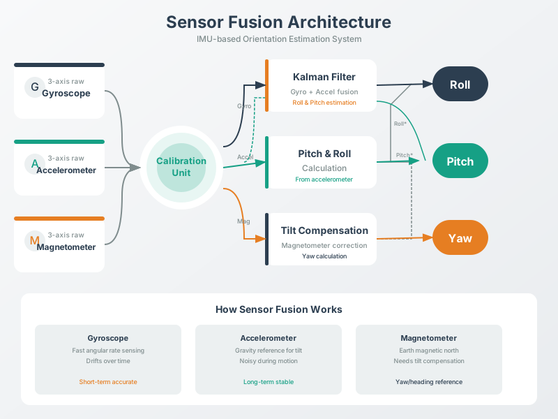
These limits explain the whole design pattern of inertial sensing: the accelerometer gives an absolute, gravity-referenced tilt that never drifts but is noisy and ambiguous under motion; the gyroscope gives smooth short-term rotation that slowly drifts. Fusing them is not a luxury — it is how you get a stable orientation from imperfect parts.
The simplest fusion logic is a complementary filter. At each sample it trusts the gyroscope for the fast change, then slowly pulls the estimate back toward the accelerometer angle: angle = alpha * (angle + gyro_rate * dt) + (1 - alpha) * accel_angle. A larger alpha follows fast rotations more smoothly but corrects drift slowly; a smaller alpha rejects drift faster but lets vibration shake the angle estimate.
Environmental pressure adds another kind of ambiguity. A BMP280 can see a floor change because pressure changes with height, but it cannot tell whether pressure changed because the device moved upward or because weather drifted over minutes. The robust lab pattern is therefore the same as IMU fusion: keep a short-term baseline, log raw and converted values, and compare the inferred event against another clue before making a decision.
Under-the-Hood Knowledge Check
37.7 Release Checklist
Before relying on motion or pressure-derived events, confirm these points:
- The IMU full-scale range, LSB-per-unit constants, raw offsets, and mounting orientation are recorded with the calibration data.
- Stationary accelerometer readings have total magnitude near 1 g, not merely near zero on each axis.
- Motion thresholds are tested across orientation changes, taps, vibration, and expected activity patterns.
- Gyroscope integrations include sample interval evidence and a drift-correction plan, such as a complementary or Kalman filter.
- Pressure-based floor or altitude logic uses a short-term baseline and relative changes rather than unqualified absolute pressure.
- Each event record stores raw values, converted units, baseline timestamp, threshold, and any companion evidence used for confirmation.
37.8 See Also
- Motion and Environmental Sensor Labs for MPU6050 and BMP280 setup, code, and exercises.
- Sensor Data Processing for filtering and confidence checks after acquisition.
- Sensor Calibration Techniques for reference records, offsets, and drift management.
- Sensor Power Management for duty-cycling IMUs and pressure sensors in battery nodes.
37.9 Next
Return to Motion and Environmental Sensor Labs once the calibration boundaries are clear, then continue to Light and Proximity Sensors for optical, PIR, ultrasonic, and capacitive readout practice.