20 Smart Agriculture: Deployment and Resilience
More
Depth: Practitioner
Progress saves as you read. Mark sections complete as you go; your progress appears in the sidebar.
- Podcast audio coming soon
- Character narration audio coming soon
20.1 Make the Irrigation Pilot Survive the Farm
Smart agriculture deployment means keeping useful farm decisions working when sensors, coverage, and field conditions change. An irrigation pilot saves water on a well-covered test block, but a full farm adds failed probes, radio shadows, livestock movement, frost risk, and changing soil. The team must design for those field failures before treating one good season as deployment proof.
Keep that team in view through the chapter. It must choose where to sample, distinguish a sick animal from a false alert, and decide which frost response the grove can actually support. A plausible reading alone cannot settle those questions: it needs calibration, a dependable field link, and a response that farm staff can carry out.
This is part 2 of 2. Smart Agriculture: Irrigation Systems and Evidence establishes the first route, including the water-savings calculation for 1,000 acres, 24 inches of seasonal water, 651.7 million gallons, and a 25% precision-irrigation scenario. Here the problem is extending a successful pilot without extending its hidden weaknesses. The approaches below begin with failure diagnosis and sensor spacing, then work through livestock, frost, connectivity, calibration, and resilient deployment.
KEY CONCEPTS
- Sensor health
Detect stuck readings before they control irrigation.
- Field coverage
Survey the sensor locations during dense crop growth.
- Individual baselines
Compare each animal with its own healthy history.
- Soil calibration
Match sensor readings to water content in each soil zone.
- Livestock biometrics
Ear tags, collars, leg bands and rumen boluses track temperature, activity, location and rumination.
- LoRaWAN gateway
Long-range field coverage depends on height, antennas, terrain, payload and duty-cycle limits.
- Frost protection
Microclimate sensors guide heating or irrigation before the crop damage threshold is reached.
20.2 Learning Objectives
By the end of this chapter, you will be able to:
- calculate sensor spacing for soil moisture monitoring
- configure livestock alerts using individual baselines
- design frost protection decisions using microclimate monitoring
- diagnose sensor and connectivity failures in field deployments
- design livestock and frost alert decisions from stated evidence
- select calibration, coverage, and recovery controls for a farm system
20.3 Diagnose Missing and Misleading Readings
Start by asking whether the pilot’s evidence is still trustworthy. Automated irrigation can waste water or damage crops when sensors fail silently and the controller keeps using stale values. Higher water bills or pump-energy costs without crop benefit are warning signs, as are waterlogged zones beside drought-stressed ones. Stuck readings do not change with weather; over-watered areas may develop root rot, fungal disease, or nutrient leaching.
Soil moisture sensors degrade through salt buildup, tillage damage, rodent damage to cables, and battery depletion. Sensor health monitoring flags out-of-range or unchanging readings instead of treating every reported number as usable. Add redundant sensors in critical zones and configure fail-safe behaviour that alerts operators rather than continuing irrigation on suspect data. During the growing season, calibrate and physically inspect sensors monthly.
Prevention also means checking plausibility: soil moisture should correlate with recent rainfall, and divergence from weather-station data should trigger an automated alert. Specify sensor self-tests and include replacement in annual maintenance budgets. Typical sensor lifespan is 2–5 years, depending on soil chemistry. Sensor Types and Biomimetic Design provides the environmental-sensor background for choosing those probes.
A missing reading presents a different diagnosis. Remote field corners may report intermittently, critical frost events, pest outbreaks, or irrigation cycles may have data gaps, and overloaded gateways may lose packets at peak transmission times. Weak signals also drain batteries through repeated retries. A gap that looks like “no change” to analytics can therefore conceal a communication failure.
Fields span hundreds of hectares with different terrain, vegetation density, and soil moisture conditions affecting radio propagation. A dormant-season trial can fail when the crop canopy develops. Conduct a radio-frequency (RF) site survey during peak growth, when vegetation is densest. Map the field topology and potential dead zones, then test every planned sensor location with portable hardware before permanent installation.
Elevated silos, poles, and pivot towers can give gateways line-of-sight coverage. Where needed, extend coverage with mesh networks or repeaters appropriate to the chosen radio system, or use a long-range protocol such as LoRaWAN. Plan a 20–30% coverage margin for seasonal change and additional sensors. A single LoRaWAN gateway cannot be assumed to cover the whole farm: terrain, vegetation, and buildings can leave blind spots, so add redundant gateways for critical sections. The vineyard example now separates a promising distance calculation from proof of field coverage.
20.4 Space Sensors Around Soil and Crop Value
The team can test its spacing assumptions with the vineyard scenario. A Napa Valley vineyard manager is deploying a precision irrigation system across a 40-hectare premium Cabernet Sauvignon vineyard with varying soil types (clay loam in low areas, sandy loam on slopes).
Given:
- Field dimensions: 800m x 500m (40 hectares)
- Soil variability: 3 distinct zones identified by soil sampling
- Vine spacing: 2m x 3m (1,667 vines per hectare)
- Water stress sensitivity: High (premium wine grapes)
- LoRaWAN gateway range: 2km line-of-sight
- Budget: $12,000 for sensors (excluding gateway)
Use the soil zones first, then adjust the layout and test its cost:
-
Apply the scenario’s initial planning density: With 3 soil zones across 40ha, each zone averages 13.3ha. A soil-moisture probe samples only its immediate location, so this worked example starts with five sensors per management zone. That is a budgeting assumption, not a statistical confidence guarantee; field calibration must use observed variability, spatial correlation, and the irrigation decision’s tolerated error.
- Minimum sensors per zone: 5
- Total minimum: 15 sensors
-
Adjust for topographic variation: Slopes cause moisture gradients. Add 2 sensors per zone for slope monitoring.
- Adjusted total: 15 + 6 = 21 sensors
-
Calculate sensor spacing: 40ha = 400,000 m². With 21 sensors: 400,000/21 = 19,047 m² per sensor ≈ 138m average spacing.
-
Verify LoRaWAN coverage: Maximum sensor distance from gateway at field center: 472m. This is within the stated 2km line-of-sight range, making a single gateway a candidate for the field survey rather than proof of coverage through terrain or canopy.
-
Budget verification: At $400-500 per sensor node (capacitive sensor + LoRa radio + solar + enclosure), 21 sensors = $8,400-$10,500. Within budget.
Result: Deploy 21 soil moisture sensors in a variable-density grid. Planning estimates in this scenario:
- Water savings: modelled as a reduction from baseline flood irrigation after calibration and valve-control checks
- Quality improvement: tighter soil-moisture control should reduce avoidable variation in grape ripening, but harvest quality still depends on weather, disease pressure, and viticulture practice
- ROI: calculate from local water cost, pump energy, labour, grape value, node cost, and maintenance rather than assuming a universal payback
Key Insight: Sensor spacing in precision agriculture is driven by soil variability and crop value, not field size alone. High-value crops like wine grapes may justify closer sensor spacing than commodity crops.
20.5 Turn Livestock Changes Into Prioritised Visits
Coverage delivers readings; useful alerting also needs a meaningful comparison. A 500-head dairy operation in Wisconsin is configuring temperature thresholds for a rumen bolus, an ingestible sensor that measures internal temperature, pH, and activity, to detect illness early while minimizing false alerts that waste veterinary time.
Given:
- Herd size: 500 lactating Holstein cows
- Normal rumen temperature range: 38.5-39.5°C (baseline varies by individual)
- Fever threshold (clinical): >39.5°C sustained for >4 hours
- smaXtec bolus accuracy: ±0.2°C
- Data transmission interval: 10 minutes
- Historical false positive rate with factory settings: 8 alerts/day (mostly false)
- Veterinary visit cost: $150 per call
- Missed mastitis case cost: $450 average (treatment + lost production)
Configure the decision around each animal rather than applying one herd threshold:
-
Establish individual baselines: Each cow has a baseline, its own normal temperature established from healthy observations. After 14-day calibration period, system calculates rolling 7-day average for each animal.
- Cow #234 baseline: 38.8°C
- Cow #456 baseline: 39.2°C
-
Configure adaptive thresholds: Rather than absolute threshold (>39.5°C for all), use deviation from individual baseline.
- Alert trigger: Baseline + 0.5°C sustained for 3+ hours
- High-priority alert: Baseline + 0.8°C sustained for 2+ hours
-
Add activity correlation: Combine temperature with activity data to reduce false positives.
- Temperature rise + decreased rumination = likely illness (priority alert)
- Temperature rise + normal activity = possible heat stress (monitor)
-
Calculate expected alert accuracy:
- With individual baselines in this scenario: false positive rate drops from 8/day to 1.5/day
- True illness detection improves because cows with lower normal baselines are no longer hidden by a herd-average threshold
- Lead time is measured against the farm’s own visual-inspection records, not assumed from the sensor alone
-
Economic validation:
- Reduced false alerts: 6.5 fewer false alerts/day × $15 labor = $97.50/day saved
- Earlier treatment: 3 additional cases caught early/month × $200 savings = $600/month
- Net benefit: ~$3,500/month improvement over factory settings
Result: Custom threshold configuration reduces false alerts in the scenario and can surface health changes earlier than visual observation when the farm validates the alert against veterinary outcomes. The annual value should be calculated from local labour, veterinary, treatment, milk-production, and herd-management data.
Key Insight: In this alert design, individual baseline calibration avoids the false positives and missed detections caused by herd-average thresholds. Each animal has a personal normal temperature range of ±0.5°C; establish that baseline while healthy and store per-animal thresholds. A temperature that indicates fever in one cow may be normal for another. Multi-sensor correlation (temperature + activity + rumination) dramatically improves alert accuracy over single-parameter thresholds.
Choosing the sensor form factor is part of the same alert decision. Continuous health and location tracking can support several farm duties:
Sensor Types:
An ear tag can combine GPS, temperature, and accelerometer readings for location, activity, and identification. A collar can add microphones to GPS and motion sensing to infer grazing behaviour, rumination, and oestrus. A rumen bolus measures internal temperature, pH, and activity over long periods, while a leg band concentrates on gait and activity signals useful for lameness detection. The correct form factor depends on the signal, attachment lifetime, animal handling, and maintenance plan.
Key Applications:
For oestrus detection, activity and rumination changes are interpreted against history so staff can prioritise checks. Calving alerts combine movement, posture, and temperature changes; illness detection looks for deviations from the individual animal’s baseline rather than only the herd average. Location data also supports grazing optimisation by showing pasture use and theft prevention through geofence alerts when an animal leaves the property.
Figure 1 answers the question farm staff actually face each morning: which of these readings is worth a visit today?
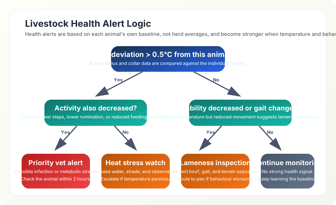
Read Figure 1 from the top box down. The first test is not an absolute temperature but a change of more than half a degree against that animal’s own baseline, which is why a naturally warm cow does not trigger a call-out. The tree then asks a second, behavioural question. A raised temperature with reduced activity leads to the tree’s vet alert within two hours, while the same temperature with normal activity becomes a heat watch: shade and water first. If the temperature is normal, the tree still checks gait, because lameness shows in movement long before it shows in heat. Every path ends in an action, including continued monitoring. The tree prioritises staff response; the worked example separately specifies how long an elevated reading must persist before its alert triggers. Patient-monitoring workflows in Healthcare IoT offer a parallel problem of turning baseline deviations into follow-up.

20.6 Knowledge Check: Agricultural IoT
20.7 Stage Frost Protection Around Forecast and Capacity
The same need to distinguish evidence from action applies to frost protection. A Florida citrus grower is deploying an IoT-based frost protection system to automate irrigation and wind machine activation across a 300-acre Valencia orange grove, protecting a $2.4 million crop from freeze damage.
Given:
- Grove area: 300 acres (121 hectares)
- Tree density: 145 trees per acre (43,500 trees total)
- Crop value: $8,000 per acre ($2.4 million total)
- Critical temperature: 28°F (-2.2°C) for 4+ hours causes fruit damage
- Frost events per season: 8-12 (December through February)
- Stated protection methods: Overhead irrigation (180 GPM/acre) and wind machines (1 per 10 acres). GPM means gallons per minute; the later 180 GPM saving calculation is a different, whole-system flow assumption.
- Current false alarm rate: 40% (unnecessary protection activations)
Separate the sensor network, forecast, response, and savings calculation:
-
Deploy microclimate sensor network:
- In-canopy sensors: 30 units at fruit height (1 per 10 acres)
- Dew point sensors: 6 units at low-lying areas (cold air pools)
- Soil temperature sensors: 6 units (thermal mass indicator)
- Wind speed/direction: 4 sensors at grove corners
- Cloud cover/sky temperature: 1 infrared sensor
- Total sensor cost: $18,500
-
Develop prediction algorithm (4-hour forecast):
- Input variables: Current temp, dew point, wind speed, cloud cover, soil temp
- Radiative cooling model: Clear sky + calm wind + low dew point = rapid cooling
- Cold air drainage model: Low-lying areas freeze 3-5°F colder than hilltops
- Prediction accuracy target: 85% for 4-hour freeze forecast
-
Configure tiered response protocol:
- Watch: at a 32°F four-hour prediction, pre-position equipment with no resource activation.
- Warning: at a 30°F two-hour prediction, start wind machines; in this scenario that means 30 machines at $85 per hour.
- Critical: at a 28°F one-hour prediction, activate irrigation only in zones whose sprinkler flow and coverage have been sized for frost protection; at 0.20 in/hour, 300 acres would need about 27,150 GPM, not 180 GPM.
- Emergency: at an actual 26°F reading, run the full protection plan.
-
Calculate resource savings from precision activation:
- Baseline unnecessary wind-machine cost: 30 hours × 30 machines × $85 = $76,500/season
- If false activations fall by 60%, wind-machine savings = $76,500 × 0.60 = $45,900/season
- Avoiding four 8-hour irrigation events at 180 GPM would save 345,600 gallons (about 0.042 acre-inches over 300 acres). This flow is too low to establish effective frost protection over the whole grove; specify protected area, required flow, and water/pumping price before assigning dollar savings.
- Damage prevention from faster response: $48,000/season
A fall from 40% to 16% false activation is a 24-percentage-point drop and a 60% relative reduction; applying 24% instead would understate the saving by $27,540.
Result: In this scenario, the IoT frost protection system delivers estimated annual benefits of $93,900:
- Wind machine fuel savings: $45,900
- Damage prevention: $48,000
- System cost: $26,500 installation + $3,500/year maintenance
- First-year payback depends on installation timing, maintenance, crop value, frost frequency, and how much unnecessary activation remains
Key Insight: Frost protection economics are dominated by false alarm costs. In this grove scenario, IoT microclimate monitoring is assumed to reduce false alarms by 60% through spatial temperature mapping that identifies which zones actually need protection, rather than treating the entire grove uniformly based on a single weather station.
20.8 Choose Connectivity at the Sensor Location
Frost response and livestock tracking make the link choice concrete: the radio must suit the location, asset movement, power supply, and payload. Use the chapter’s comparison ranges as planning inputs, then verify the actual site. LPWAN Fundamentals compares low-power wide-area network options.
| Link | Chapter planning figures | Farm role |
|---|---|---|
| LoRaWAN | 2–15 km; 5–10 year battery targets; 0.3–50 kbps | Soil sensors and weather stations. |
| Sigfox | 10–50 km; 100 bps payloads | Simple status sensors where a Sigfox network is available. |
| NB-IoT | Cellular-coverage range; 5–10 year battery targets; roughly 100 kbps | Livestock tracking where carriers cover the farm. |
| Satellite | Global reach; 1–10 kbps | Remote ranches, with careful message-frequency, terminal-cost, and battery design. |
| Wi-Fi | 50–100 m; high data rates | Barns and greenhouses with local power. |
LoRaWAN often fits fixed field sensors because a self-deployed gateway can cover large open areas when link budget, antenna height, terrain, and crop canopy allow it. Small payloads and infrequent reporting support multi-year battery targets, especially for Class A devices that mostly sleep. Unlicensed spectrum avoids carrier contracts but still requires regional frequency planning and duty-cycle awareness. Node costs depend on enclosure, sensor quality, power system, certification, installation labour, and support model. LoRaWAN Network Architecture explains the network behind that choice.
Figure 2 returns to the vineyard so the range claim stays tied to an actual field layout.
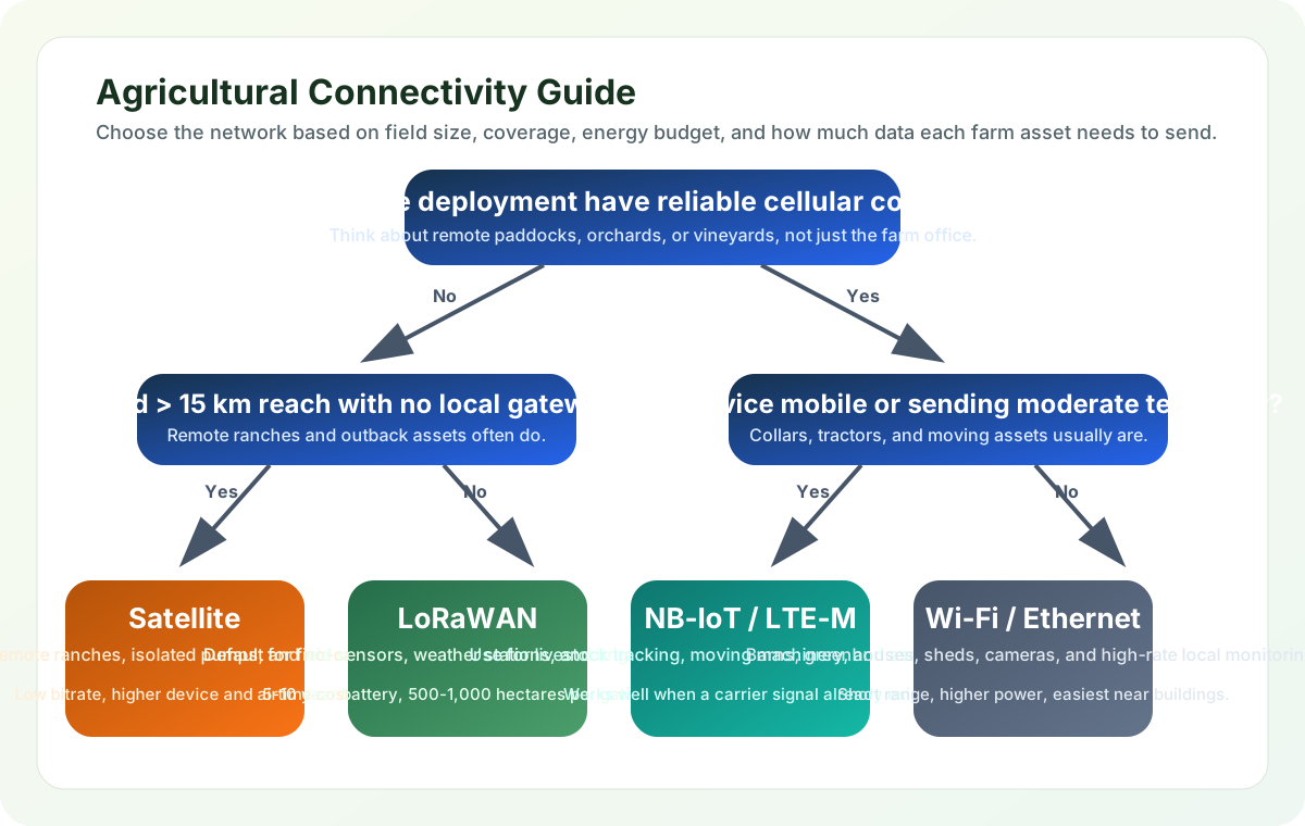
Start with coverage in the fields and barns rather than at the farm office. Without cellular service, compare the required field distance with a private LoRaWAN gateway design; beyond about fifteen kilometres, satellite becomes an option to assess. With carrier coverage, moving assets such as collars and tractors can use suitable low-power cellular links, while fixed barn cameras may use Wi-Fi. These are starting choices: each depends on its measured coverage and power plan.
The gateway’s route onward also matters. The chapter connects sensors (Module 2), LoRaWAN (Module 4), and edge processing (Module 5). Edge/Fog Computing explains on-farm processing that can reduce cellular costs. Smart Grid gives the related rural-energy-management context. Neither a reachable gateway nor a local processor fixes an uncalibrated probe, which is the next boundary to check.
20.9 Calibrate the Soil Before Setting Thresholds
A working radio can faithfully deliver the wrong moisture interpretation. A capacitive soil moisture sensor uses the surrounding soil’s dielectric properties to estimate water content. Using the manufacturer’s default calibration curve for irrigation decisions can misstate actual volumetric water content (VWC), the proportion of soil volume occupied by water.
Why This Happens: Soil moisture sensors ship with a generic calibration (often for sandy loam or laboratory test media). Different soil types — clay, silt, sand, organic matter — have vastly different dielectric properties, meaning the same sensor reading (say, 50% VWC) corresponds to completely different actual moisture levels in clay versus sandy soil.
Scenario: A California almond grower deploys 80 capacitive sensors across a 100-hectare orchard with mixed soil types:
- Zone A (sandy loam): Sensor reads 35% VWC, actual VWC = 32% (close enough)
- Zone B (clay loam): Sensor reads 35% VWC, actual VWC = 48% (13 percentage points above the reading)
- Zone C (sandy): Sensor reads 35% VWC, actual VWC = 22% (13 percentage points below the reading)
The grower set a “below 30% VWC” irrigation threshold based on Zone A. The shared 35% reading would not trigger that rule in any zone, yet Zone C is actually at 22%. These readings show why the common threshold can miss dry sandy soil; they do not alone establish that the clay zone was over-watered. Without soil-specific calibration, already-wet clay can receive unnecessary irrigation and sandy zones can suffer avoidable stress, depending on the bias and control rule.
Why Soil Type Matters: The chapter’s illustrative dielectric ranges explain why a generic curve needs testing; they do not replace a measured calibration curve or establish one bias direction for every sensor.
- Pure sand: a low dielectric constant, around 3-5, can make water look artificially dry.
- Clay: a high dielectric constant, around 15-25, can make soil look wetter than it is.
- Organic matter: variable dielectric behavior, often around 10-20, is unpredictable without calibration.
- Saline soils: very high conductivity and dielectric effects can cause severe moisture over-reading.
The remedy is a zone-specific comparison with measured water content. Use the following workflow when the generic curve cannot support the irrigation decision.
Proper calibration workflow:
- Soil Sampling: Collect representative soil samples from each zone (3-5 zones per field based on soil survey maps)
- Lab Analysis: Send samples for texture analysis (sand/silt/clay percentages)
- Gravimetric Calibration:
- Take soil cores next to installed sensors at 5 different moisture levels
- Weigh wet and dry at 105°C for 24 hours, measure dry bulk density, and convert gravimetric water content to actual VWC
- Record sensor readings at each actual moisture level
- Generate zone-specific calibration curve
- Adjust Sensor Firmware: Apply zone-specific calibration coefficients to sensor nodes
- Validation: Repeat spot-checks monthly during first season
Quick Field Check (if lab calibration isn’t feasible):
- Irrigate a small test area to field capacity (soil saturated, then drained)
- Wait 24 hours, take sensor reading
- Simultaneously take a soil core, measure wet/dry mass and dry bulk density, then calculate actual VWC
- Calculate offset: Actual VWC - Sensor VWC = Correction factor
- Apply correction to all sensors in that zone
Cost-Benefit:
- Lab calibration: $200-400 per zone (3-5 samples)
- Improves irrigation decisions by separating actual soil-water status from sensor bias
- For a 100-hectare farm, calibration value should be estimated from local water price, pumping energy, crop value, and the cost of wrong irrigation decisions
Key Warning Signs Your Sensors Need Calibration:
- Sensors in different field zones show identical readings despite visible moisture differences
- Irrigation controllers never reach your set thresholds (always “too dry” or “too wet”)
- Some zones develop root disease (over-watering) while others show drought stress (under-watering)
- Sensor readings don’t respond to rainfall within 24 hours
Prevention: Always specify “soil-specific calibration” in procurement contracts. Budget $50-100 per sensor for calibration — cheaper than one failed crop or wasted water season.
20.10 Make the Deployment Sequence Reviewable
Bring spacing, calibration, connectivity, and staff response back into one deployment sequence. Conduct a soil survey to identify distinct zones, install and calibrate sensors with soil-specific curves, then collect baseline data over 2–4 weeks to establish normal moisture patterns. Configure irrigation thresholds and variable-rate application maps only after that evidence is available. Monitor crop response and refine sensor density using yield data.
Variable-rate application adjusts fertiliser, pesticide, or water dosage by field zone. It depends on trustworthy maps and equipment as well as sensors. Higher-value crops can justify denser grids; lower-margin commodity crops usually need simpler instrumentation. The vineyard’s five-per-zone starting point remains a budgeting assumption, so refine it against observed variability and the decision’s tolerated error.
Keep the farm loop’s responsibilities visible. Field sensing binds a calibrated reading to its plot, depth, and time. The farm gateway carries that reading while preserving plot, sensor, and timestamp context. Irrigation decision and actuation combines the evidence with policy, commands the valve, and records what happened. Separating these responsibilities lets the grower trace a bad decision to sensing, context transfer, or actuation logic.
For livestock, validate early alerts against veterinary outcomes and tune staff workflow to avoid alert fatigue. For frost, preserve the distinction between a forecast target, an activation rule, and protection equipment sized for the affected zone. For irrigation, a calibration budget and redundant coverage are part of the operational design, alongside power and local fallback. A deployment is useful when the grower can act on the evidence in time.
Summary
Smart agriculture creates value when calibrated measurements change farm decisions. Sensor health checks expose stuck or implausible values; peak-season surveys expose coverage gaps. Sensor density follows soil variability and crop value rather than field area alone. Individual animal baselines and correlated activity signals help staff prioritise checks, while microclimate forecasts support staged frost protection within actual equipment capacity.
Match each radio to field coverage, data rate, reporting interval, power, and maintenance. Apply soil-specific calibration before production thresholds and calculate benefits from local water, energy, labour, treatment, and crop data. Together, those choices connect a successful test block to a farm system whose failures can be diagnosed.
Agricultural IoT succeeds when sensing, connectivity, power, and farm operations are designed together. A technically accurate reading is valuable when it reaches the grower in time to change irrigation, fertilisation, disease response, or equipment use.
Next, Smart Manufacturing carries these concerns into industrial IoT, predictive maintenance, and supply-chain visibility.