5 IoT Domain Requirements: Latency, Scale, and Power
More
Depth: Practitioner
Progress saves as you read. Mark sections complete as you go; your progress appears in the sidebar.
- Podcast audio coming soon
- Character narration audio coming soon
5.1 Let the Field Limit Shape the Design
An IoT requirement states what a system must do in its operating setting, and what evidence will show that it does it. This chapter turns domain differences into latency, downtime, scale, availability, and battery calculations. Those calculations help locate the system boundary before a team chooses its radio, protocol, or cloud platform.
Picture three teams buying the same connected unit. A farmer wants ten years between battery visits. A hospital wants a warning before a patient is harmed. A factory wants a machine stopped before a tool breaks. The same feature list cannot prove all three jobs: the consequence of a late, lost, wrong, or exposed result changes the design.
The chapter’s Sensor Squad makes the differences concrete. Thermo the Temperature Sensor monitors a sick child in hospital. In this example, Thermo samples every second and must get fever alerts to a nurse within seconds. Medical-grade equipment and a strong Wi-Fi connection are candidate provisions; their presence alone does not prove that the whole alarm path meets its requirement. Hydro the Humidity Sensor watches a vineyard for frost. The scenario treats frost as developing over 30 minutes, permits checks every few minutes, and targets a 10-year battery and a $50 unit because the farmer needs hundreds. LoRaWAN carries small messages over long distances. Motion Mo the Motion Detector works in a self-driving car with a response target below 10 milliseconds. That target leaves little time for a cloud round trip, so processing must stay inside the vehicle. A hospital patient monitor may target 99.99% availability and sub-second alerts; determine clinical, privacy, power, and cost requirements for each deployment.
These are example requirements to test, rather than guarantees attached to a technology name. Thermo’s hardest limit is dependable warning; Hydro’s is service life across distant fields; Mo’s is response time. The problem is choosing an architecture that can prove its particular claim. We will first write a requirement envelope, then compare timing and outage budgets, and finally test how scale and power narrow the available approaches.
Latency is the time from an event to the result that needs it. State the limit for each traffic class instead of calling the whole design real time. Bandwidth is how much data a link can carry in a given time. Count message size, send rate, device count, bursts, updates, and retries; a calm average can hide the hour when every unit reports at once. Test the narrowest shared link. A protocol is an agreed set of rules for an exchange. Choose those rules after power, range, message, delay, and ownership needs are clear.
The comparison spans six dimensions: latency, reliability, scale, power, data volume, and regulation. We will use them to match technology choices to domain constraints and evaluate trade-offs. Regulation also changes project cost and timeline through review, evidence, and support obligations; the next chapter develops data and regulatory selection in more detail.
KEY CONCEPTS
- Latency budget
Set the latest useful response for the domain.
- Power budget
Sampling and radio duty cycle constrain service life.
- Scale boundary
Device count changes addressing, updates, and support.
5.2 Learning Objectives
By the end of this chapter, you will be able to:
- Compare domain requirements across latency, reliability, scale, power, and data volume dimensions
- Explain regulatory impacts on IoT project cost and timeline
- Match technology choices to domain-specific constraints
- Evaluate trade-offs when selecting IoT solutions for different applications
5.3 Domains Turn Ideas Into Constraints
A requirement envelope records the decision, tight constraints, flexible constraints, and rejection tests for a domain. Healthcare, agriculture, transportation, smart homes, smart cities, and factories can all use sensors, gateways, networks, and dashboards, but the acceptable latency, reliability, power budget, data volume, regulation, and maintenance model are different because the consequence of failure is different. A few seconds of delay in a smart-home leak alert may be acceptable if the device has multi-year battery life. The same delay in an industrial safety interlock or clinical alarm can be unacceptable because the user expects a local, auditable, fail-safe response.
The envelope names the decision the IoT system supports, the constraints that are tight, the constraints that are flexible, and the trade-off that would make the application unsafe, unaffordable, or unmaintainable. It prevents a team from starting with a favorite radio, cloud platform, or dashboard and then forcing every domain to fit it. A farm frost monitor, a cold-chain shipment tracker, a city parking sensor, and an OPC UA-connected factory asset monitor may all report telemetry, but they do not carry the same response time, uptime, calibration, evidence, privacy, and support obligations.
Use the envelope as a comparison artifact:
- Healthcare monitoring: Safety workflow, privacy, identity matching, and auditability usually tighten first, so strong identity, retained evidence, and clinical integration such as HL7 FHIR can matter before dashboard features.
- Agriculture: Range, battery life, weather exposure, and seasonal maintenance usually tighten first, so LPWAN options such as LoRaWAN or cellular IoT may matter before visual analytics.
- Industrial automation: Uptime, deterministic response, asset context, and plant integration usually tighten first, so edge control, Ethernet, OPC UA, MQTT Sparkplug, or ISA-95 alignment may dominate.
If a requirement is tight, the design needs evidence: a latency budget, a battery calculation, a site survey, a retention rule, a failover test, or a maintenance plan. If a requirement is flexible, the design should say what flexibility is being used to reduce cost or complexity. That discipline makes later technology choices defensible instead of accidental.
5.3.1 Start With the Tightest Constraint
The first stop is the eliminator: the requirement that rules out the most tempting but unsuitable design before the team spends time polishing it.
For project work, start with the hardest constraint and let it narrow the design. A vineyard frost sensor may eliminate high-power radios before data modeling matters because replacing batteries across distant fields is expensive and time-sensitive. A hospital monitor may eliminate best-effort connectivity before cost optimization matters because missed identity, delayed escalation, or unclear alarm ownership can create clinical risk. A factory control loop may require local edge control, deterministic networking, OPC UA context, or ISA-95 integration before cloud analytics is useful because production equipment cannot wait for a remote dashboard to decide whether a machine should stop.
Write the envelope with measurable language. Latency should name the response window, such as sub-second local action, under ten seconds for an operator alert, or daily reporting for planning. Reliability should name what happens during packet loss, gateway outage, drained battery, sensor fault, or unavailable cloud service. Scale should name device count, site count, onboarding rate, and replacement workflow. Power should name battery life, duty cycle, sleep behavior, and access for maintenance. Data should name sample rate, units, timestamp source, quality flags, retention, aggregation, and whether raw data or events must be preserved. Regulation and governance should name consent, tenant boundaries, audit logs, export controls, privacy reviews, or safety evidence when those apply.
Only then compare candidate technologies. LoRaWAN Class A can be attractive for low-rate, battery-powered field sensors, but it limits downlink behavior and payload size. NB-IoT or LTE-M can remove gateway ownership for wide-area assets, but carrier coverage, SIM lifecycle, and recurring cost become requirements. Wi-Fi may suit mains-powered indoor devices with existing site networks, but provisioning and IT approval can dominate deployment. BLE may fit phone-assisted setup or local wearables, while Ethernet may fit industrial panels where power and cabling are available. MQTT, CoAP, HTTPS, OPC UA, and MQTT Sparkplug are not interchangeable labels; each brings different assumptions about message delivery, semantics, tooling, and integration.
End the practitioner pass with evidence tests. A good envelope points to a site survey, link-budget check, battery calculation, protocol trace, environmental test, accessibility review, security review, pilot success metric, or support drill. If the technology survives the test tied to the domain decision, it is a candidate. If it only works in a clean demo, the envelope has exposed the risk early.
5.4 Requirement Envelopes as Contracts
The deeper reason domain requirements matter is that they assign responsibility across the system. A latency requirement decides what must run on the device, gateway, edge server, cloud service, and user interface. A reliability requirement decides redundancy, watchdogs, monitoring, queueing, retry limits, idempotency, and failover. A regulation requirement decides identity, logging, retention, consent, deletion, audit boundaries, and who can view or export data. Without that allocation, the architecture may look complete while nobody owns the requirement when the deployment fails.
Consider a latency envelope. The user-facing number is not a single network measurement; it is the sum of sensor sampling, firmware filtering, radio wake time, gateway processing, broker delivery, stream processing, notification, and human response. If a factory interlock must act locally, the cloud may only record evidence after the fact. If a parking sensor can tolerate minutes, the design may batch messages to save power. If a medical alert has a safety escalation path, the system must distinguish a normal reading, stale reading, rejected reading, offline device, and acknowledged alarm because each state has a different operator meaning.
Reliability and data quality also cross layers. MQTT QoS can reduce message-loss risk, but it does not prove that the sensor was calibrated, the unit is correct, the timestamp is trustworthy, or the command is safe to retry. Store-and-forward can protect against outages, but the application still needs stale-data labels and sequence handling. OPC UA information models or MQTT Sparkplug birth certificates can preserve asset and tag context in industrial systems, but the receiving historian, rules engine, and dashboard must retain that meaning. Healthcare or regulated deployments may need patient or device identity matching, audit logs, and retention rules before data can enter clinical or compliance workflows.
For deeper review, test the envelope against failure modes: offline gateway, stale sensor, drained battery, delayed alert, duplicate command, denied credential, changed regulation, unavailable cloud service, bad calibration, and expensive maintenance visit. The test is not whether the page still draws a chart. The test is whether the system still supports the domain decision safely, visibly, and with enough evidence for the responsible operator. If the design still holds under those conditions, the technology choice is defensible. For a control action, say what safe state remains when the result is unknown. Test a lost link, dead unit, wrong time, full store, and late message. Show doubt instead of guessing.
5.5 Build a Requirement Envelope
To write the envelope, name the decision and who depends on it. Rank all six dimensions as tight, moderate, or flexible; identify the eliminator; compare radios, protocols, compute placement, storage, and operations against the same limits; and write the evidence test before deployment. Include outcome, scale, place, power, time, data, loss, safety, privacy, support, cost, owner, and rejection test on one page.
5.6 Requirement Progression
A smart-home leak sensor puts battery life, clear local alerts, and low maintenance first: a few seconds may be tolerable, but missed alarms damage trust. A cold-chain shipment monitor must also balance cellular or LPWAN coverage, temperature accuracy, tamper evidence, and exception reporting. A factory safety interlock makes deterministic response, local fail-safe action, maintenance ownership, and audit evidence hard constraints before dashboards or predictive analytics.
These comparisons are useful even at home. A smoke detector carries life-safety consequences; a doorbell can often tolerate a few seconds; and a thermostat may tolerate hours offline, depending on its setting. The acceptable outage follows the supported job, rather than the label “smart device.” The vehicle analogy follows the same logic: healthcare resembles an ambulance, agriculture a rugged, efficient tractor, autonomous control a precise race car, and household monitoring an affordable bicycle. Each serves a different job, so speed or price alone cannot rank them.
The six questions put ranges on the comparison: how fast, from milliseconds to hours; how available, from 95% to 99.999% uptime; how many devices, from 10 in a house to 50,000 across a city; which source of power, from a wall outlet to battery or solar; how much data, from a few bytes to gigabytes per day; and which government rules or safety standards apply. Answering them first can prevent months of unsuitable development and narrow hundreds of options to a working shortlist of roughly 3–5 candidates. The shortlist still needs evidence.
5.7 Domain Requirement Envelopes
The layered workflow in Application Domain Requirements Contracts extends this envelope into latency, reliability, power, security, data, lifecycle, governance, and integration budgets.
5.8 The Healthcare vs Agriculture Comparison
The envelope becomes easier to judge when two teams measure the same quantity. Compare Thermo’s patient-monitoring task with Hydro’s vineyard task; their numbers below are illustrative design targets.
Consider two temperature monitoring scenarios that illustrate how the same measurement can have completely different requirements:
Hospital Patient Monitoring
- What’s measured: Patient body temperature
- Criticality: Life-threatening if measurement is missed or inaccurate
- Response needed: Immediate (seconds) for fever alerts
- Accuracy required: +/-0.1C (medical-grade precision)
- Reliability: 99.99% uptime (lives at stake—52 minutes downtime per year maximum)
- Compliance: HIPAA (patient data privacy), FDA (applicable medical-device review)
- Cost tolerance: $500+ per sensor acceptable (patient safety justifies expense)
Vineyard Frost Monitoring
- What’s measured: Air temperature in agricultural fields
- Criticality: Crop damage if frost missed, but not life-threatening
- Response needed: Minutes (frost builds slowly over 30-60 minutes)
- Accuracy required: +/-1C (frost threshold is approximately 0C)
- Reliability: 95% uptime acceptable (redundant sensors compensate for failures)
- Compliance: No medical-device compliance assumed in this agricultural example; applicable radio, site, and data obligations still need review
- Cost tolerance: <$50 per sensor (need hundreds, agriculture has tight margins)
Same measurement (temperature), completely different requirements!
This comparison reveals why domain requirements matter: the consequences of failure, the speed of decision-making, regulatory oversight, and economic constraints all vary dramatically based on context.
Figure 1 puts a number range behind each requirement. That is what turns the patient-monitor and vineyard comparison into a design brief.
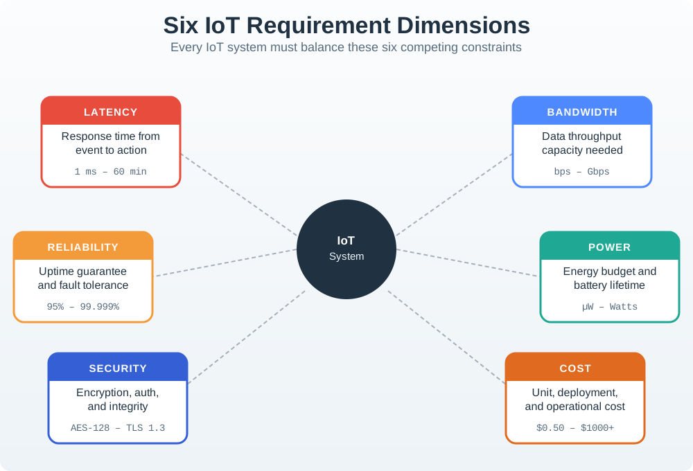
The six panels in Figure 1 surround one system, and the ranges under each name are the useful part. Latency spans a millisecond to an hour, so fast enough means nothing until the domain names its own limit. Reliability runs from 95 percent to five nines, which is the gap between a spare sensor and a second network. The comparison also spans costs from fifty cents to a thousand dollars per unit. Read the six dimensions together: power can constrain the response rate, while regulation can change the evidence and support the architecture needs. Neither the unit price nor a radio name settles the whole design.
5.9 Latency and Response Time
Different applications have fundamentally different time constraints based on what they’re controlling and the consequences of delays:
A given delay has different consequences across the domains in Figure 2 because their response limits differ.
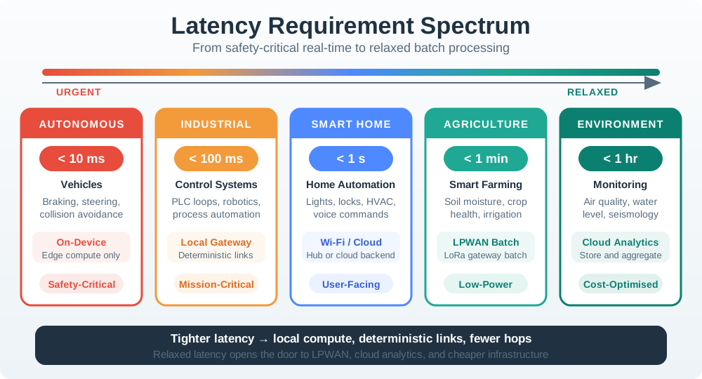
Compare the two end points first. Then place each workload. Read Figure 2 from the under-10-ms vehicle limit through industrial robotics, building automation, agriculture, and hourly environmental monitoring. As the physical process changes more slowly, the response budget relaxes and cloud processing becomes more plausible. A 100 ms delay equals 0.1 s: it is ten times a 10 ms vehicle limit and can be catastrophic at road speed, yet it consumes only one thirty-six-thousandth of a one-hour environmental window. Architecture follows that consequence. Tight safety loops stay local; tolerant monitoring can trade delay for wider aggregation and simpler operations.
- Autonomous vehicles: Under 10 ms because avoiding collisions at highway speeds leaves almost no cloud round-trip budget.
- Industrial robotics: Under 50 ms because precise assembly operations require real-time coordination.
- Building automation: Under 1 second because HVAC response and lighting adjustments need to feel immediate to users.
- Smart agriculture: Under 1 minute because irrigation decisions are based on slowly changing soil conditions.
- Environmental monitoring: Under 1 hour because weather and air quality change gradually over time.
Key Insight: A 100 ms delay is catastrophic for autonomous vehicles but completely acceptable for environmental monitoring. Understanding these latency requirements drives architecture decisions—autonomous vehicles need edge computing (local processing), while environmental monitoring can use cloud platforms.
5.10 Latency-to-Distance Tool
The distance tool separates the arithmetic from a safety claim. It converts mph to metres per second with a factor of 0.44704, converts milliseconds to seconds, and multiplies speed by delay. Metres convert to feet with a factor of 3.28084. Distance travelled during processing is only one part of a vehicle’s response; a latency threshold alone cannot establish collision-avoidance safety.
5.11 Downtime Cost Spectrum
System reliability requirements directly correlate with the human and economic cost of failure:
Inspect Figure 3 to translate four example uptime targets into downtime and the controls needed to meet them.
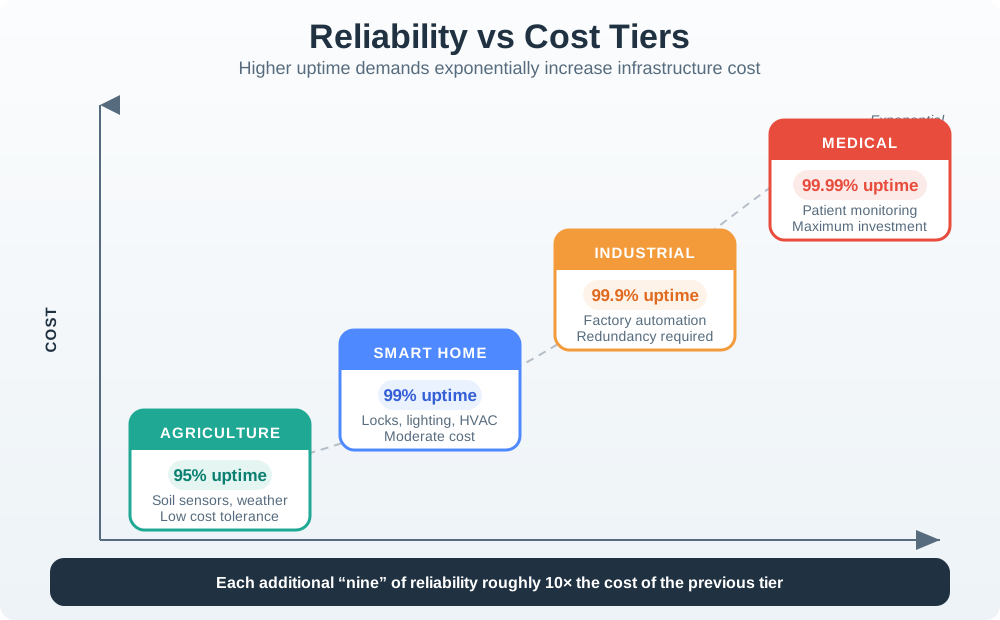
Read Figure 3 from the 95% agriculture example to the 99.99% healthcare example. Five percent of a 365-day year is 18.25 days, which matches the roughly 18 days shown for the first target; four nines permit only about 52 minutes. The consequences also change, from recoverable inconvenience to traffic disruption or patient harm. The lower downtime is not bought as a percentage. It comes from independent failure domains, failover, monitoring, spares, maintenance, and tested recovery, each priced against the service consequence.
The percentages in Figure 3 are example service targets, not domain-wide requirements. The cost multipliers shown are also assumptions for a hypothetical design exercise. Real targets and costs come from the service’s harm model, operating window, failure dependencies, recovery time, staffing, and supplier commitments. In this comparison, healthcare uses 99.99% uptime, or at most about 52 minutes of downtime per year, because failure can harm patients. Traffic control uses 99.9%, or about 8.7 hours, because failure can cause accidents, disruption, and economic loss. Smart home uses 99%, or about 3.6 days, where failure is usually an inconvenience. Agriculture uses 95%, or about 18 days, for a scenario in which redundancy or manual response can recover some losses.
Real-World Implications:
Achieving 99.99% uptime generally requires redundancy, failover, continuous monitoring, and tested recovery, so the harm model must justify that infrastructure. A smart-home user may tolerate an occasional thermostat outage, whereas traffic control requires stronger failure isolation and recovery. There is no universal cost multiplier for each additional “nine”; the architecture and its common-cause failures determine the actual cost.
5.12 Reliability Cost Reasoning
Consider two services with 10,000 sensors. One can tolerate a day-long outage during a non-critical operating window; the other must continue through a gateway, power, or network failure and restore service within minutes. The percentage targets describe outcomes, but they do not price the designs.
Build the estimate from concrete controls:
- identify independent failure domains, including power, gateways, backhaul, cloud services, and field devices
- decide which failures require redundancy and whether failover is automatic
- include monitoring, spares, maintenance access, incident response, and recovery testing
- model common-cause failures so duplicated components are not mistaken for independent protection
- price the complete service boundary, then test whether the proposed design can meet its target
A $50,000 baseline and a 99.99% target are therefore insufficient to calculate a hospital-system price. Two architectures with the same target can have very different costs and failure behaviour.
5.13 Interactive: Availability Budget Calculator
The availability calculator translates targets of 95%, 99%, 99.9%, 99.99%, and 99.999% into annual outage budgets. On a 365-day basis those budgets are 18.25, 3.65, 0.365, 0.0365, and 0.00365 days respectively. It deliberately does not estimate cost: the percentage supplies neither the architecture nor the operating model. Specify which failures must be prevented or recovered within the budget, then price those controls.
5.14 Scale From Wearables to Cities
Latency and uptime decide response architecture; scale and power decide whether that architecture can be deployed and maintained in the real world.
Deployment scale fundamentally changes system architecture, cost structure, and technology choices:
- Personal, 1-10 devices: Fitness trackers and smartwatches usually use Bluetooth to a smartphone and need no site infrastructure.
- Home, 10-50 devices: Smart-home automation usually uses Wi-Fi or Zigbee mesh, a single gateway, and a consumer budget.
- Building, 50-500 devices: Office HVAC and security deployments need a building-wide network, IT staff, and professional installation.
- Campus, 500-5,000 devices: Universities, hospitals, and vineyards need dedicated network infrastructure plus gateway management.
- City, 5,000+ devices: Municipal parking and streetlights usually need LoRaWAN, NB-IoT, a city-scale backbone, and an operations center.
Technology Selection by Scale:
- Personal/Home (1-50 devices): Bluetooth, Wi-Fi, Zigbee (existing consumer infrastructure)
- Building/Campus (50-5,000 devices): Wi-Fi, LoRaWAN gateways, wired Ethernet (dedicated infrastructure)
- City (5,000+ devices): LoRaWAN, NB-IoT, or Sigfox. Check provider coverage where available; a private LoRaWAN deployment needs gateways, backhaul, and operations.
5.15 Power Source Drives Everything
The availability of power fundamentally constrains connectivity and sensor choices:
- Mains power: Continuous external power supports Wi-Fi, Ethernet, video, and high-power sensors in buildings, traffic cameras, and industrial deployments.
- Power over Ethernet: External power over network cabling supports IP cameras, VoIP devices, and Wi-Fi access points in offices and warehouses.
- Rechargeable battery: One to seven days between charges supports Bluetooth and moderate sensors in wearables, smartphones, and patient monitors.
- Long-life battery: One to ten years supports LoRaWAN, NB-IoT, and ultra-low-power sensors in parking and environmental monitoring.
- Solar plus battery: A ten-or-more-year service target supports LoRaWAN, Sigfox, and periodic sampling in agriculture and remote environmental sites.
- Energy harvesting: Operation depends on enough ambient energy being available, supporting BLE beacons and low-power sensors in indoor tracking or maintenance-free niches.
Example: Why agriculture uses LoRaWAN instead of Wi-Fi:
- Wi-Fi: the example assumes 100–200 mW transmit power and battery depletion in weeks; actual service life also depends on duty cycle and the complete power budget
- LoRaWAN: in this example, assume 20–50 mW transmit power and a ~200 ms uplink every 10 minutes (about 0.03% transmit duty cycle); estimate battery life from the complete power budget
- Result: $50 sensor with 10-year battery vs. $200 sensor + solar panel or frequent battery replacement
A complete power budget records every state in a normal day and a bad day: sleep, wake, sense, send, listen, retry, update, and recover. Use measured current and time rather than assigning battery life from the radio label. Add the travel and labour needed to replace a battery; a low-cost unit can create an expensive maintenance route.
5.16 Interactive: Battery Life Estimator
The battery estimator uses a simplified two-state model. It multiplies capacity in mAh by an assumed 3.7 V to obtain mWh, then weights transmit and sleep power by their time fractions. Battery energy divided by average power gives hours; divide by 24 for days and by 365 for years. Its controls span 10–250 mW transmit power, 0.01–10% duty cycle, capacities of 1,000, 2,000, 3,000, 5,000, or 10,000 mAh, and 0.001–5 mW sleep power. Starting values are 50 mW, 1%, 3,000 mAh, and 0.05 mW. Treat the result as a screening estimate: the full state budget still has to support the service-life claim. A lifetime result alone cannot select LoRaWAN, Sigfox, NB-IoT, Bluetooth LE, or rechargeable Wi-Fi without the other envelope constraints.
5.17 Radio Remi’s Math Bridge: Band Choice and Reporting Duty
The reporting-duty calculation shows why the time fraction matters. At equal distance, 915 MHz saves 8.38 dB of free-space loss relative to 2.4 GHz. Dropping transmit power from 150 mW to 35 mW gives up 6.32 dB, leaving a net 2.06 dB in LoRaWAN’s favour under those assumptions. A 200 ms report every 10 minutes is active for 0.0333% of the time, rather than 1%, producing about 12.3 microamps average and an 8.42-year derated service-life screen.
Before extending the deployment, run a small pilot against the tightest limit. For battery life, measure the worst radio day. For delay, load the shared path. For audit evidence, trace one fact and one action from source to record. Keep both pass and fail evidence, and keep the pilot small enough to change when the field contradicts an assumption.
Give the envelope to another team, a field worker, and the person who pays. Ask each to identify the hardest limit and the evidence that could reject the plan. If their answers differ, resolve the missing fact or unclear service promise before buying more parts. Reopen the record when the site, regulation, device count, software, or service promise changes; a design that fits today may fail at the next scale.
Summary
A requirement envelope ties the domain decision to measurable timing, availability, scale, power, data, and regulatory constraints. Thermo, Hydro, and Motion Mo illustrate why the same connected-device feature list cannot prove every job. Start with the tightest limit, eliminate unsuitable options, and ask for the evidence that remains missing.
Latency allocates work between local processing and remote services. Availability allocates failure controls and recovery obligations, whose costs must be estimated explicitly. Scale adds infrastructure and support work; power turns reporting behaviour into a maintenance commitment. The final choice should state the claim, limit, owner, rejection test, and what remains unknown.
Choose technology only after the domain’s hardest constraint has a measurable limit and a test that could reject the design.