19 Smart Agriculture: Irrigation Systems and Evidence
More
Depth: Practitioner
Progress saves as you read. Mark sections complete as you go; your progress appears in the sidebar.
- Podcast audio coming soon
- Character narration audio coming soon
19.1 Choose Whether to Water the Dry Patch
Smart agriculture uses field and animal sensors to turn changing conditions into timely farm actions. Water, soil, weather, labour and market timing can change faster than a fixed schedule can handle. The useful result is a decision to irrigate, feed, spray, move, repair or wait, with evidence that the action helped. This first of two chapters builds that decision loop, follows the precision-agriculture stack and tests irrigation evidence.
Imagine a grower sees one dry patch while rain is due later that day. The grower must choose whether to water now, wait or inspect the field. Telemetry means reports that a device sends so people can check conditions from afar. A soil report gives the grower another pair of eyes, but the dry patch does not describe the whole field.
19.1.1 Check the Crop Zone
Begin with the crop zone and the probe’s location. Compare nearby readings and expected rain, check that measurements are current and in the expected units, then decide whether to operate the valve. Keep probe location, reading time, weather context and the valve decision together. If the probe is stale or its link is lost, show that uncertainty and use the grower’s inspection path.
19.1.2 When One Probe Is Not Enough
One moisture reading cannot establish conditions across different soil patches. Assess coverage by management zone, soil type and slope, retaining installation depth and calibration with each reading. After irrigation, check valve state and flow confirmation alongside the subsequent moisture response. If the response disagrees with expectations, review installation, calibration and placement as well as the valve. The problem is therefore larger than detecting dryness: the grower needs a trustworthy path from a local observation to an action and its physical result. The approaches below build that path.
Farmer Emma’s Sunny Acres Farm offers a simple illustration of why local measurements matter. In the Sensor Squad story, Thermo finds soil at 45 degrees overnight, below the story’s 55-degree tomato target, even though the air feels warm. These temperatures are in degrees Fahrenheit and illustrate the story’s conditions rather than a universal crop rule. Sunny the Light Sensor finds that an oak tree shades one cornfield corner in the afternoon, where plants grow more slowly. Moisture Monitor finds 15% moisture in Section 3 and 45% in Section 7: the two sections do not call for the same watering. Power Pete connects those observations to tiny solar panels and efficient batteries intended to support years of field operation. Crop monitoring checks plant conditions across rows; livestock tracking follows animals’ location and health. Each observation is useful only when Emma can decide what to do with it.
We will trace a vineyard’s sensor reading through calibration, transmission, recommendation and valve feedback, then calculate a corn farm’s water-saving scenario. Sensor spacing, individual livestock thresholds, frost decisions and deployment pitfalls remain part of the wider agriculture route; here the emphasis is the irrigation loop and the evidence it must preserve.
19.2 Key Concepts
KEY CONCEPTS
- Precision agriculture
Site-specific management varies inputs by field zone, rather than treating the whole field uniformly.
- Soil moisture
A capacitive probe measures water as a percentage of soil volume and needs soil-specific calibration.
- Variable-rate application
VRA adjusts fertiliser, pesticide or water to sensor-mapped spatial variability.
- Agronomic threshold
A crop-specific trigger, such as soil moisture below 25%, starts irrigation or a farmer alert.
19.3 Learning Objectives
By the end of this chapter, you will be able to:
- Explain the precision agriculture IoT stack from sensing to actuation
- Decide whether to irrigate from a probe reading when rain is due
- Check valve state and flow confirmation
- Estimate water savings
19.4 Define the Farm Action Before Choosing Sensors
A smart agriculture system is useful only when it changes a farm action: irrigate a zone, open a greenhouse vent, treat an animal, move a herd, protect a crop from frost, service a pump, or hold off on applying fertiliser. The sensor is not the product by itself. The product is the decision loop that connects field conditions to timely action.
For a soil-moisture deployment, the irrigation loop includes calibrated capacitive readings of volumetric water content (VWC), the percentage of soil volume occupied by water, or tensiometer readings of soil-water tension, alongside soil texture, root-zone depth, crop growth stage, weather forecast, irrigation valve state, flow confirmation, and a way for the operator to override the recommendation. For livestock, it includes animal identity, normal baseline, tag or bolus health data, activity change, location, and a veterinary workflow that makes the alert actionable.
Figure 1 follows a soil reading into an irrigation decision. Keep its context attached across each boundary.

Start the loop with calibrated capacitive or tensiometer readings in a named field zone. Soil texture, root depth, and crop stage give that number agronomic meaning before LoRaWAN carries it through the gateway. Cloud analysis adds weather, and the dashboard presents a recommendation with an operator override. A command then opens a zone valve, but the loop is not closed until valve state and flow confirm that water moved. Field identity, calibration context, and action evidence must survive every boundary or a correct reading can still irrigate the wrong place.
The loop uses four physical things that are easy to picture wrongly: a probe in the soil, a node that sends its reading, a valve that opens, and a meter that confirms water moved. The four photos below show a typical example of each.
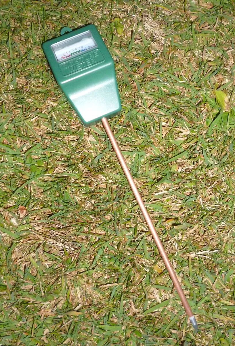
Note where the prong enters the ground. A probe measures only the soil next to it, which is why the chapter places probes by management zone rather than one per field.
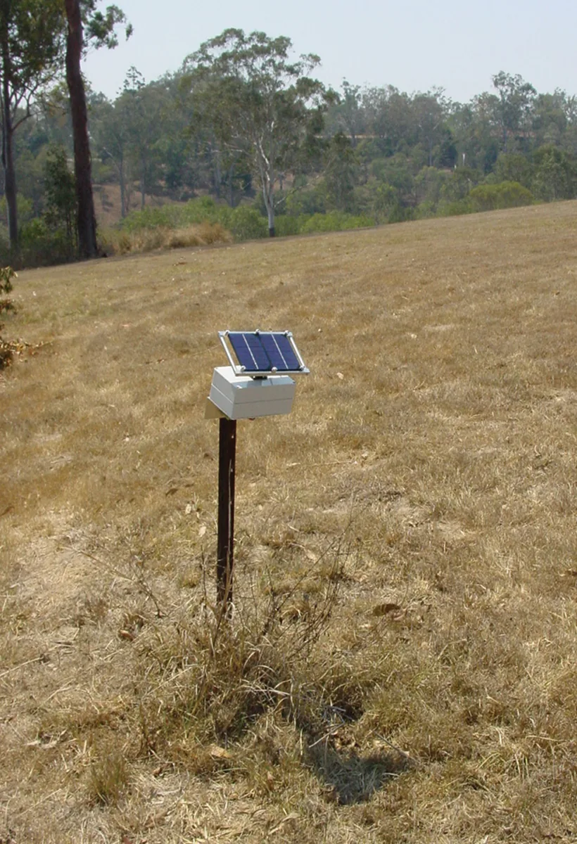
The node is small and sits on a stake beside the probe. It is the part that carries "Sensor #23" onto the LoRaWAN link.
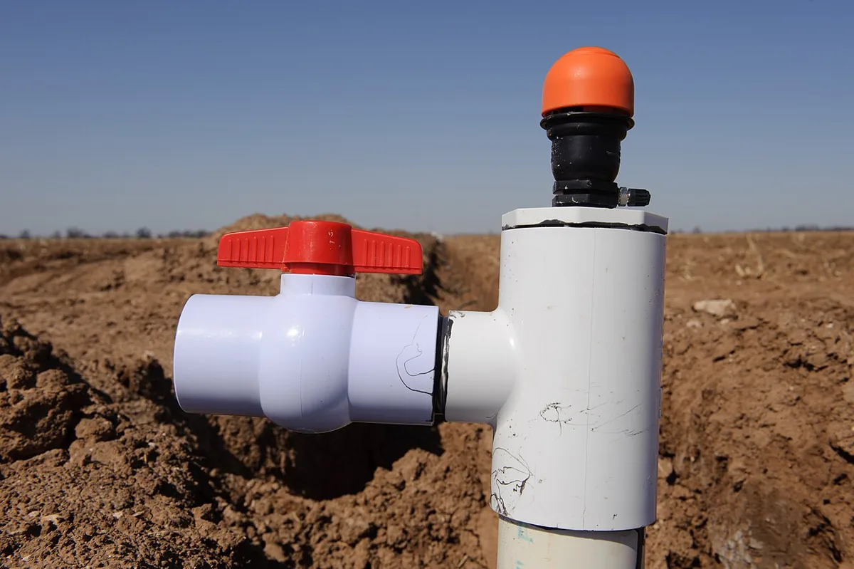
The valve is the actuator. The system sends the command, but the loop is not closed until valve state is confirmed.
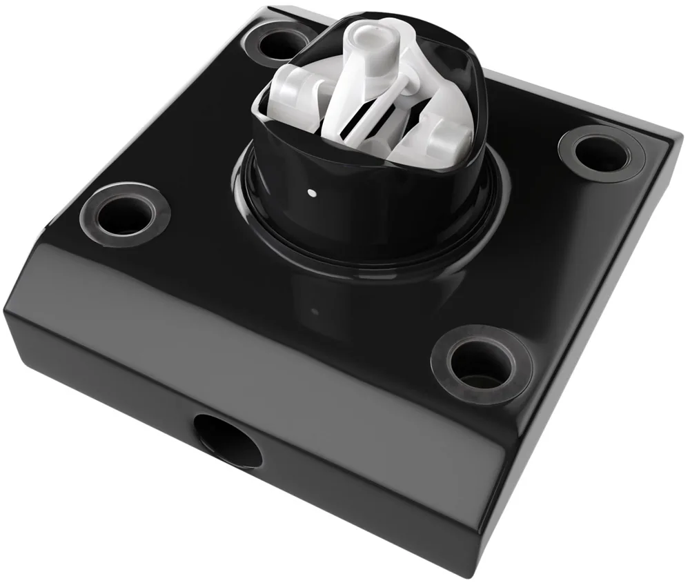
Read the "flow confirmation" in the farm loop as this: after the valve opens, a flow reading above zero proves water is moving. A valve that reports open with no flow may be blocked or the supply may be off.
- Field crops: place sensors by management zone, soil type, slope, and crop value rather than by a simple grid.
- Livestock: treat tags, collars, leg bands, and rumen boluses as baseline trackers, not standalone diagnosis devices.
- Controlled environments: connect temperature, humidity, CO2, light, substrate moisture, vents, heaters, and irrigation setpoints into one control model.
The beginner mistake is to treat agriculture IoT as a hardware shopping list. The useful framing is narrower: define the agronomic decision, name the data needed before the decision, name the action after the decision, and prove that the loop changes yield, input use, labor, welfare, compliance, or risk. A dashboard that reports conditions after the crop is stressed is monitoring; a system that changes the irrigation or treatment plan in time is operational IoT.
19.5 Map the Field, Season and Evidence
Start with a map of the operation. Mark soil zones, pump locations, valve groups, power sources, gateway candidates, barn walls, canopy height, low frost pockets, animal routes, and places where workers already inspect equipment. That map determines whether LoRaWAN, NB-IoT/LTE-M, BLE tags through readers, Wi-Fi, private cellular, or satellite backhaul is the right fit.
The field map answers where devices belong; the seasonal map answers when they can be made trustworthy. Installation and baseline learning need time before the first operational decision.
A practitioner should also map the season. Installation before planting, sensor calibration during wet and dry conditions, gateway surveys before canopy growth, and actuator testing before irrigation demand are different tasks. If the deployment waits until the crop is already stressed, there may be no safe opportunity to tune thresholds. For livestock, baseline learning needs enough normal days to separate illness, heat stress, calving, feeding changes, and ordinary movement patterns. Calibrate thresholds per animal rather than relying only on a herd average: a temperature signalling fever in one cow may be normal for another. Interpret it with activity, rumination, location and recent heat stress.
- Choose the decision threshold. Define what reading changes action, such as volumetric water content below a crop-stage threshold, rumination dropping from an animal baseline, or leaf-wetness duration crossing a disease-risk rule.
- Prove the measurement. Calibrate soil sensors against gravimetric samples, verify temperature probes in the installed enclosure, check antenna RSSI/SNR at crop height, and record battery behavior under the chosen reporting interval.
- Close the loop. Confirm that valve state, pump current, flow meter pulses, tag check-ins, or greenhouse actuator feedback show whether the command actually changed the physical system.
The implementation details matter. A LoRaWAN Class A soil node that sends a 12-byte payload hourly has a different power and latency profile than a cellular cattle collar with global navigation satellite system (GNSS) fixes, or a greenhouse controller using Modbus, MQTT, or OPC UA over wired Ethernet. Design each data path around the farm action it supports.
Commissioning should produce evidence, not just installed devices. Keep a gateway coverage map, a sensor calibration record, a threshold rationale, a battery-life estimate, and an operator escalation path. Test failure modes deliberately: blocked gateway antenna, dead battery, stuck valve, missing animal tag, stale weather feed, and a sensor that flatlines after being dislodged. The farm team needs to know whether the system will fail safe, alert a person, or continue with conservative defaults.
19.6 Agriculture Data Needs Context
Those commissioning records need to travel with the readings. Agricultural telemetry is easy to misread when context is stripped away. Store the sensor identifier, calibration curve, soil zone, installation depth, units, timestamp, battery state, firmware version, quality flag, and nearby weather station context with each reading. For geospatial data, preserve coordinates, field boundary, management zone, and equipment pass when data flows into a time-series store or farm-management platform.
Connectivity and power choices also shape the data model. LoRaWAN often suits low-data-rate field sensors because the farm can deploy its own gateway. NB-IoT/LTE-M, Wi-Fi, BLE, private cellular or satellite may suit animals, machinery, barns, greenhouses or remote properties better. LoRaWAN airtime and duty-cycle limits favor compact, infrequent telemetry. NB-IoT and LTE-M support wider coverage where cellular service exists but add carrier dependency and power budget pressure. BLE livestock tags may need barn readers or mobile gateways. Satellite can cover remote ranches but changes message frequency and cost assumptions. None of these technologies removes the need for calibration, identity, and physical confirmation.
- Identity: bind every sensor, valve, animal tag, gateway, and actuator to the field, herd, or zone it claims to represent.
- Quality: flag stale values, impossible jumps, flatlined sensors, missed packets, and readings outside calibrated range before analytics use them.
- Control: separate recommendation, command sent, command acknowledged, actuator moved, and physical effect confirmed as different states.
Real deployments often combine farm systems with general IoT infrastructure. ChirpStack or a carrier LoRaWAN network server may feed MQTT, HTTP webhooks, AWS IoT Core, Azure IoT Hub, TimescaleDB, InfluxDB, or a farm-management platform. The integration should preserve units, timestamps, field identity, and quality flags across those systems. If the time-series database stores a number but drops the calibration curve or field boundary, downstream dashboards may look precise while making unsafe agronomic recommendations.
Under the hood, a field reading is rarely a single number. A moisture value may need raw sensor counts, calibration version, soil temperature, installation depth, salinity warning, last rainfall, irrigation event id, and the management zone boundary used by the control rule. A livestock event may need animal id, device placement, firmware, last gateway contact, activity window, baseline model version, and whether staff confirmed the animal was checked. Without that metadata, analytics can confuse a bad sensor with a dry field or a missing tag with a healthy animal.
The probe and the radio path also respond to water. In the vineyard example, the far corner is 471.7 m away. At 915 MHz, free-space loss is 85.1 dB. A vegetated-path exponent of 2.8 raises the modelled loss to 106.5 dB, leaving 46.5 dB from a 153 dB link budget. Water and dry soil also differ in permittivity: that contrast shifts a capacitive probe’s oscillator by about 8.5% between 25% and 30% water content. These calculations connect plot geometry, canopy loss, fade margin, dielectric mixing and oscillator response.
19.7 Follow Sensor #23 to the Valve
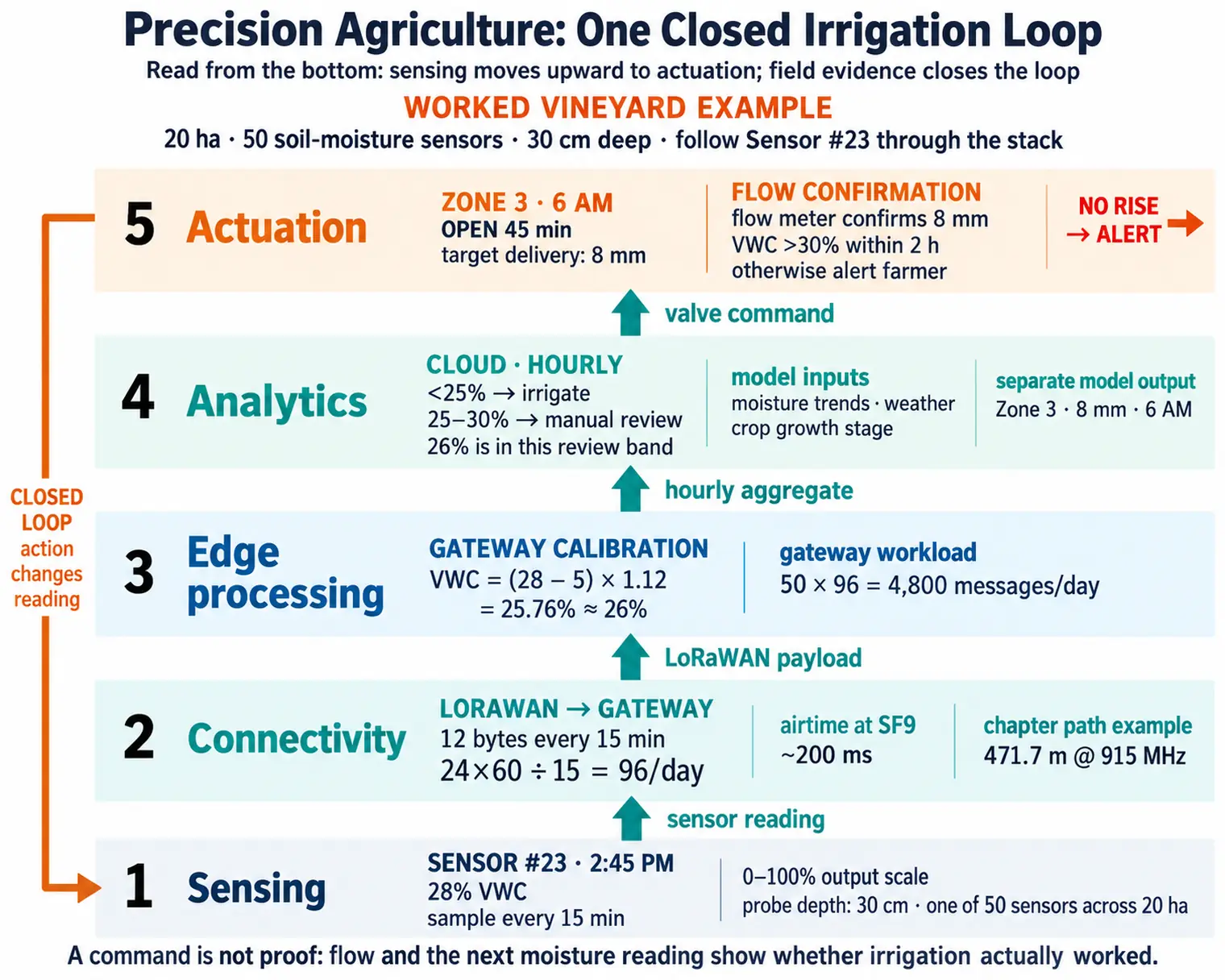
The earlier problem now has a concrete field loop. The vineyard has 50 soil-moisture sensors buried 30 cm deep across 20 hectares. Each measures VWC every 15 minutes. At saturation, VWC is approximately the soil’s porosity, rather than 100%. Sensor #23 reports raw 28% VWC at 2:45 PM.
LoRaWAN carries each 12-byte payload to a gateway in the equipment shed. A reading every 15 minutes means 96 messages per day per sensor and 4,800 messages per day across the 50 sensors. The example uses about 200 ms airtime per transmission at spreading factor 9 (SF9) and a projected 5–7 years on one 3.6 V lithium cell. Treat that lifetime as the example’s estimate alongside the reporting interval and deployment power budget.
At the gateway, edge logic applies soil-specific calibration: VWC_actual = (VWC_raw - 5) × 1.12. Sensor #23’s raw 28% becomes 25.76%, rounded to 26%. The system alerts below 25% VWC or above the soil-specific saturation or waterlogging threshold. The 25–30% band calls for manual review, so 26% does not automatically trigger the below-25% rule.
The cloud receives hourly aggregates, while field sampling remains every 15 minutes. A machine-learning model combines current moisture trends, temperature and rainfall forecasts, and crop growth stage; the example notes greater water needs for flowering vines. Its recommendation is: “Zone 3 needs 8 mm irrigation tomorrow at 6 AM.” The manual-review step lets the operator assess that recommendation before scheduling it.
At 6 AM, the system commands Zone 3’s solenoid valve to open for 45 minutes. The flow meter must confirm delivery equivalent to an 8 mm water depth. Sensor #23 should then rise above 30% VWC within two hours. If it does not, the farmer receives an alert for a possible sensor-burial or valve fault. Actuation changes the next readings, which inform the next decision; without that feedback, irrigation would remain a fixed schedule regardless of soil conditions.
Installation can break this loop even when the electronics work. An air gap around Sensor #23 can produce a reading of 15% VWC while the soil is saturated. Responding with more water wastes it and risks root rot. Installation quality therefore matters as much as sensor technology.
Keep one action record that another person can audit: Sensor #23, vineyard Zone 3; calibrated 26% VWC at 2:45 PM; irrigation below 25% with manual review at 25–30%; scheduled 8 mm at 6 AM; required flow-meter confirmation; and a follow-up rise above 30% within two hours. This keeps the threshold, command and validation signal together. If the result disagrees with the model, the team can investigate calibration, placement or the valve using that record.
19.8 Connect the Stack to Farm Operations
The stack builds on earlier agricultural technology. Ploughs, GMO crops and GPS tractors improved production while data often stayed in separate systems. Weather stations, soil sensors and plant monitors provide real-time environmental streams, but those streams can overwhelm farmers without interpretation. Unmanned aerial vehicle (UAV) drones, AI analytics and autonomous equipment can turn measurements into recommendations when connectivity and skills are in place. The operational gain comes when the farm uses those recommendations in time.
- Sensing: soil-moisture probes, sap-flow sensors, and weather stations show when and where irrigation is needed.
- Connectivity: LoRaWAN, satellite, and other links move field readings across large properties with few gateways when the link budget allows it.
- Analytics: edge and cloud models can predict yield risk or disease pressure when they keep calibration and field context.
- Actuation: variable-rate irrigation and drone spraying apply inputs only where the farm has evidence to act.
- Integration: farm-management software brings sensor, equipment, and operating records into one decision surface.
For larger farms, the integration layer is often a context platform rather than a single dashboard. A gateway may translate field protocols into a shared model, a context broker may keep the latest state for fields, sensors, pumps, animals, and equipment, and an export service may archive selected records for research or compliance. FIWARE NGSI-LD, Open Geospatial Consortium (OGC) SensorThings, MQTT topic contracts, or farm-management APIs can all support that pattern when the record still preserves device identity, location, timestamp, unit, calibration state, and the rule that changed an irrigation or husbandry decision.
Figure 2 shows where a soil reading has to travel before it can change how much water a field gets.
Read Figure 2 from the bottom. The sensing layer gathers soil moisture, weather, canopy images and livestock data, so the record starts with field context rather than a dashboard. Connectivity then splits by asset: wide fields ride LoRaWAN, moving equipment rides cellular, and satellite fills the gaps. Analytics sits above that, where gateway filters drop noise and cloud models estimate irrigation, disease and frost risk. Actuation turns those estimates into valve, drone and alarm commands. The arrow that closes the loop is the important one. Every action changes the next set of readings, so the farm has to judge the stack by what the following week measures.
The economic claims need the same field evidence:
- Precision irrigation can reduce avoidable watering when the baseline system over-irrigates or misses field-zone differences
- Variable-rate fertiliser and pesticide programs can reduce input waste when maps, calibration, and application equipment are trustworthy
- Yield benefits depend on crop stress, weather, disease pressure, soil variability, and whether the farm changes operations in time
- Cost savings should be estimated from the farm’s water price, pump energy, labour, crop value, equipment cost, and maintenance burden
19.9 Livestock and Controlled Ag
The feedback pattern also applies beyond irrigation. Agricultural IoT often moves beyond field irrigation into animal health and climate-controlled production:
- Rumen bolus monitoring places an ingestible sensor in cattle to track stomach temperature, pH, activity, and rumination. Value comes from detecting fever, acidosis, or heat stress 24-48 hours before visible symptoms, but thresholds must be tuned per animal to avoid false alerts.
- Greenhouse climate control combines temperature, humidity, CO2, light, and substrate-moisture sensors with heating and ventilation commands. The ROI depends on closing the loop: sensor reports must lead to action, whether automated or taken by an operator, to produce savings.
- Poultry-house monitoring watches ammonia, floor-level temperature, humidity, and ventilation balance. Small feed conversion ratio improvements compound quickly at flock scale, so sensor placement must capture microclimates at bird height rather than only ceiling conditions.
Start with the farm decision that changes action, such as treating an animal, opening a vent or irrigating a zone, then work backward to sensor placement, connectivity, power budget, and alert thresholds.
19.10 Estimate Water Savings Before Claiming Them
Let’s calculate a scenario for water savings from precision irrigation on a corn farm:
Given: A 1,000-acre corn field using flood irrigation applies 24 inches of water per growing season.
Volume calculation:
- Baseline seasonal water volume: 1,000 acres x 24 inches x 1 foot / 12 inches x 43,560 square feet per acre = 87.12 million cubic feet.
- Gallon conversion: 87.12 million cubic feet x 7.48 gallons per cubic foot = 651.7 million gallons.
- Precision-irrigation scenario: 25% savings x 651.7 million gallons = about 163 million gallons saved per season.
- At an assumed agricultural water cost of $0.002 per gallon, the scenario saves about $326,000 per season.
Treat that as a worked estimate: the real result depends on local water pricing, pumping energy, crop response, and whether the control loop prevents both over-watering and under-watering.
19.11 Summary
Precision agriculture varies treatment by field zone, using measurements that retain location, calibration, time and quality context. The vineyard example follows Sensor #23 from raw 28% VWC to about 26%, manual review, an 8 mm command and independent confirmation through flow and moisture response. The stack is useful when those steps change timely farm action.
Farm economics depend on crop value, baseline practice, water price, pump energy, labour and maintenance. The corn example’s 25% saving is a scenario to test against the farm’s actual results. Livestock and controlled environments require the same discipline: meaningful baselines, suitable placement and evidence that action followed the reading.
Design the farm decision first, then preserve the evidence from calibrated measurement through physical action and its result.
Carry this decision loop into Smart Agriculture: Deployment and Resilience to examine sensor spacing, livestock thresholds, frost protection and field failures.