32 Predictive Maintenance: Models and Rollout
32.1 Start With the Story
A vibration model can flag a bearing pattern, but some failures appear first as heat and every alert must still become a planned job. The team now has to combine evidence, choose a model, and connect each warning to an economic and operational rollout decision.
32.2 Overview
This route adds thermal imaging and model selection, then carries alerts into work orders, ROI, rollout, and context-aware operation.
This is part 2 of 2. Review Predictive Maintenance: Signals and Vibration when you need the first route.
32.3 Learning Objectives
By the end of this chapter, you will be able to:
- combine thermal and vibration evidence for maintenance decisions
- select a machine-learning model with stated operating limits
- connect alerts to work orders, ROI evidence, and staged rollout
32.4 Chapter Roadmap
Follow the original sections below in order. They begin at the reviewed split boundary and keep every worked example, figure, check, and supporting banner with the section that owns it.
32.5 Thermal Imaging
Infrared cameras detect thermal anomalies:
Look at Figure 32.1 for the tool an inspector actually carries on a route, and for what it cannot do.

Look first at the body in Figure 32.1. It is a pistol grip with a trigger, built to be aimed one-handed while the other hand holds a torch or a clipboard. The screen sits above the grip, so a reading is checked at the asset rather than back at a desk. The lens at the front sets the field of view, which decides how close an inspector must stand to a live panel. Nothing here records a route on its own. That is the limit the rest of this section builds on: a handheld sweep is a snapshot taken by a person, so repeatable trending needs a fixed sensor or a strict capture procedure.
32.5.1 Thermal Monitoring Architecture
Figure 32.2 answers what the camera alone cannot: how a hot reading turns into an action.
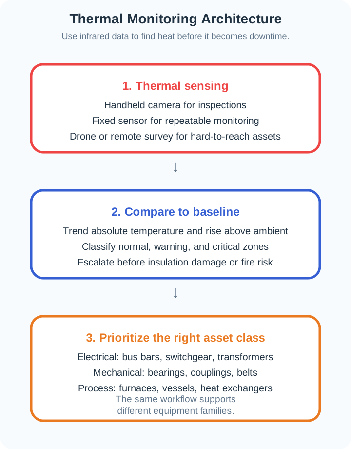
Read Figure 32.2 downward in three moves. The top band is sensing, and it already forces a choice: a handheld camera suits an inspection route, a fixed sensor suits repeatable trending, and a drone survey suits assets nobody can reach safely. The middle band is where a temperature becomes evidence, because a reading only means something next to a baseline and the rise above ambient. That comparison sorts a site into normal, warning and critical. The bottom band then aims the effort at bus bars, bearings or heat exchangers. The same three steps serve all three families, so the workflow is reusable even when the failure physics differ.
Thermal monitoring architecture showing infrared sensing technologies feeding into analysis engine for baseline comparison, trending, and anomaly detection across electrical, mechanical, and process equipment applications.
32.5.2 Electrical Applications
- Hot spots on connections indicate high resistance
- Overheated components indicate overload
- Phase imbalance in motors
- Can detect problems 6-12 months in advance
32.5.3 Mechanical Applications
- Bearing overheating (friction)
- Belt misalignment (heat buildup)
- Lubrication issues (dry bearings)
- Coupling problems
32.5.4 Temperature Thresholds
| Component | Normal | Warning | Critical |
|---|---|---|---|
| Motor bearings | <70°C | 70-85°C | >85°C |
| Electrical connections | <40°C rise | 40-70°C rise | >70°C rise |
| Gearbox oil | <80°C | 80-95°C | >95°C |
32.6 Machine Learning Models
Vibration and thermal rules handle many faults directly. When conditions vary by load, recipe, season, and maintenance history, ML can help, but only if the model choice matches the evidence you actually have.
Modern predictive maintenance uses ML to learn normal behavior and detect anomalies.
32.6.1 ML Model Selection Decision Tree
Figure 32.3 sorts model families by the labels you hold, not by the algorithm you like.
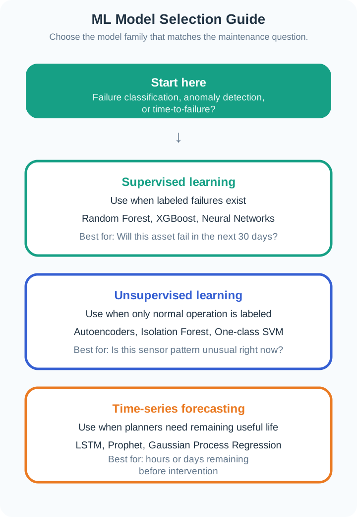
Begin at the question box in Figure 32.3, which asks what the maintenance team needs to know. The three branches below answer it in the order of evidence you can supply. Supervised learning comes first, and it needs labelled failures, which many sites do not have. Unsupervised learning needs only a record of normal running, so it suits a plant with clean history and few recorded faults. Forecasting sits last because it needs runs that were followed all the way to failure, the hardest data of all. Each branch also states its own question: will this asset fail soon, is this pattern odd now, how long is left.
Use this decision tree to select the appropriate ML approach based on your available data and prediction goals.
32.6.2 Supervised Learning
Approach: Requires labeled failure data to train classifiers.
Algorithms:
- Random Forest, XGBoost for classification
- Neural networks for complex patterns
Output: “Will this bearing fail in next 30 days?” (Yes/No with probability)
Requirements:
- Historical failure data (dozens to hundreds of examples)
- Consistent sensor data leading up to failures
- Domain expertise to label failure modes
32.6.3 Unsupervised Learning
Approach: Learns normal operation without failure labels.
Algorithms:
- Autoencoders (reconstruction error indicates anomaly)
- Isolation Forests (detects outliers)
- One-class SVM
Output: “Is this vibration signature abnormal?” (Anomaly score)
Advantages:
- Works without historical failures
- Detects novel failure modes
- Good for rare events
32.6.4 Time-Series Forecasting
Use this time-series forecasting section as a guided decision record, not as a list to memorise. First identify the stated input, assumption, or scenario; then compare each option on the same units and time boundary. Next check which value changes the outcome and which evidence would reveal an invalid assumption. For time-series forecasting, the useful result is the reasoning chain: observed condition, governing constraint, calculation or classification, and operational consequence. Record that chain before choosing an answer or carrying a value into the next section. Where the panel supplies several choices, reject each distractor against the chapter’s named mechanism instead of relying on wording cues. Where it supplies a table or timeline, compare rows at like-for-like scale and preserve the difference between an early indication, an actionable threshold, and a final outcome. This turns time-series forecasting into evidence that can be reviewed, recalculated, and connected to the running design narrative.
Approach: Predicts remaining useful life (RUL) based on degradation trends.
Algorithms:
- LSTM neural networks
- Prophet (trend + seasonality)
- Gaussian Process Regression
Output: “How many hours/days until failure?” (RUL estimate with confidence interval)
Key metrics:
- Mean Absolute Error (MAE)
- Root Mean Square Error (RMSE)
- Percentage within 10%/20% tolerance
 Checkpoint: Model Choice
You now know:
- Supervised learning can answer whether a bearing will fail in the next 30 days, but it needs labeled failure examples.
- Unsupervised anomaly detection can start from normal operation only, but it still needs engineer review before action.
- RUL and time-series models estimate time to failure only for the asset class, fault mode, and operating context represented in the training data.
32.7 Alert to Work Order
An automotive smart-factory maintenance program usually succeeds or fails at the handoff between analytics and maintenance execution. The useful case-study pattern is not “AI predicted a fault” by itself; it is a closed loop from condition evidence to work order, inspection, repair, and model feedback.
Example scope:
- Critical conveyors, robots, compressors, pumps, spindles, and drives are ranked by failure impact.
- Vibration, current, temperature, cycle-count, and controller-state data are captured with asset id, speed/load context, and maintenance history.
- Edge gateways compute features near the machine while historians, OPC UA servers, MQTT brokers, or MES/CMMS connectors move selected evidence upward.
- Maintenance planners review severity, confidence, spare-part lead time, and production windows before scheduling work.
What to measure:
- Alert precision and missed-fault rate by failure mode.
- Time from first warning to confirmed inspection.
- Planned work percentage versus emergency work percentage.
- Downtime avoided, repair hours, spare-part waste, and technician trust.
Figure 32.4 shows where an alert stops being an analytics output and becomes scheduled work.

Follow the numbered loop in Figure 32.4. The first two stages are the part most teams build first: capture the signal with its load context, then compare features against a baseline. The third stage decides whether the system is trusted, because an engineer can reject a bad alert before it costs a shift. Stages four and five turn a confirmed fault into a repair booked against spare-part lead time and a production window. The dashed return is why this is drawn as a loop rather than a line: technician outcomes go back into thresholds and models. The band underneath lists what each pass must leave behind.
The workflow must leave an auditable trail. Each alert should identify the asset, feature values, baseline comparison, severity, recommended inspection, technician disposition, replaced part, and return-to-service result.
Lesson learned: Success requires maintenance adoption, not just analytics. Technicians need enough evidence to challenge bad alerts, confirm real faults, and feed the outcome back into thresholds and models.
Highly automated electronics plants often use the same building blocks discussed in this chapter: PLCs and PROFINET or industrial Ethernet at the machine layer, OPC UA or historian interfaces for operations data, RFID or traceability records for product context, and analytics that compare equipment behavior against known-good baselines.
Integration pattern:
- Production equipment emits process values, alarms, cycle counts, and quality results.
- Asset health features are tied to product, recipe, shift, maintenance event, and environmental context.
- Quality, maintenance, and operations teams review the same asset history rather than separate dashboards.
- Digital twin or simulation work is used for what-if planning, not as a replacement for measured condition data.
Business impact to verify locally:
- Fewer emergency repairs on critical bottleneck assets.
- Higher planned-maintenance ratio without excessive part replacement.
- Lower false-alarm burden for technicians.
- Better root-cause records for repeat failures.
Key Success Factor: The plant treats PdM as a maintenance decision system with measured outcomes, not as a standalone ML demo.
32.8 ROI Calculation Framework
32.8.1 Cost Components
Investment costs (illustrative ranges; replace with local quotes):
- Sensors: $100-500 per motor (vibration, temperature)
- Gateways: $500-2,000 per zone
- Software: $50,000-500,000 (depending on scale)
- Integration: 2-5x hardware cost for brownfield
- Training: $1,000-5,000 per technician
Operating costs (illustrative ranges; replace with local contracts):
- Platform licensing: $10-50 per asset/month
- Connectivity: $5-20 per gateway/month
- Data storage: $0.02-0.05 per GB/month
- Analyst time: $50,000-100,000/year for dedicated resources
32.8.2 Benefit Categories
Direct savings:
- Reduced emergency repairs (labor + parts + expediting)
- Extended equipment life (deferred replacement)
- Lower spare parts inventory (order when needed)
- Reduced energy consumption (efficient equipment)
Indirect savings:
- Avoided production losses (unplanned downtime)
- Improved quality (equipment in specification)
- Reduced safety incidents (early warning of hazards)
- Better capital planning (known equipment condition)
32.8.3 Sample ROI Calculation
Use this sample roi calculation section as a guided decision record, not as a list to memorise. First identify the stated input, assumption, or scenario; then compare each option on the same units and time boundary. Next check which value changes the outcome and which evidence would reveal an invalid assumption. For sample roi calculation, the useful result is the reasoning chain: observed condition, governing constraint, calculation or classification, and operational consequence. Record that chain before choosing an answer or carrying a value into the next section. Where the panel supplies several choices, reject each distractor against the chapter’s named mechanism instead of relying on wording cues. Where it supplies a table or timeline, compare rows at like-for-like scale and preserve the difference between an early indication, an actionable threshold, and a final outcome. This turns sample roi calculation into evidence that can be reviewed, recalculated, and connected to the running design narrative.
Scenario: 100-motor manufacturing plant using editable planning assumptions.
| Item | Value |
|---|---|
| Average motor replacement cost | $15,000 |
| Historical failures per year | 8 |
| Average downtime per failure | 12 hours |
| Downtime cost per hour | $5,000 |
| Annual failure cost | $600,000 |
With predictive maintenance:
The table’s $180,000 investment is a separate case from the interactive calculator’s $140,000 default; the calculator does not reproduce this table unless its investment inputs are aligned.
| Item | Value |
|---|---|
| Investment (sensors, software, integration) | $180,000 |
| Annual operating cost | $36,000 |
| Failure prediction rate | 85% |
| Prevented failures | 6.8 per year |
| Annual savings | $510,000 |
| Payback period (after annual operating cost) | 4.6 months |
Interactive element unavailable — chart cell
Plot: Observable Plot (charting library) is not bundled
Show source
html`<div style="margin: 20px 0;">
<h4 style="color: #2C3E50;">Investment Breakdown</h4>
${Plot.plot({
marginLeft: 100,
x: {label: "Cost ($)", grid: true},
y: {label: null},
marks: [
Plot.barX(roiBreakdown, {
y: "category",
x: "cost",
fill: "#3498DB",
tip: true,
title: d => `${d.category}: $${d.cost.toLocaleString()} (${d.percent}%)`
}),
Plot.text(roiBreakdown, {
y: "category",
x: "cost",
text: d => `$${(d.cost/1000).toFixed(0)}K`,
dx: -30,
fill: "white",
fontSize: 12,
fontWeight: "bold"
}),
Plot.ruleX([0])
]
})}
</div>`You now know:
- The sample 100-motor case uses 8 historical failures, 12 hours per failure, $5,000 per downtime hour, 85% prediction, and a 4.6-month payback after annual operating cost.
- The separate chemical-plant example pays back in about 9 months after subtracting $50,000/year operating cost from prevented-failure savings.
- Phase 1 should select 10-20 high-criticality assets, prove at least one previously undetected issue, and expand only after technician-confirmed alert quality.
32.9 Implementation Roadmap
Inspect Figure 32.5 to see what each rollout stage must prove before more assets are added.
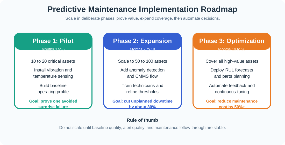
Prove one asset first. Expand only after measured value. Read Figure 32.5 from the 10–20-asset pilot to expansion and facility coverage. The pilot installs basic sensing, builds normal baselines, and must catch one previously unseen issue. Expansion to 50–100 assets adds anomaly models, CMMS work orders, and technician training; success is a measured drop in emergency work on those asset classes. Only then does the final stage add remaining-life forecasts, parts automation, and continuous model improvement. Coverage grows after alert quality and maintenance follow-through are stable, not simply when the model emits more warnings.
Implementation timeline showing three phases: Pilot (months 1-6) focuses on critical asset selection and baseline establishment, Expansion (months 7-18) scales coverage and adds ML capabilities, and Optimization (months 19-36) achieves full facility coverage with automated workflows.
32.9.1 Phase 1: Pilot (Months 1-6)
- Select 10-20 critical assets
- Deploy basic vibration and temperature sensors
- Establish data collection infrastructure
- Create baseline normal operation profiles
- Success metric: Detect one previously undetected issue
32.9.2 Phase 2: Expansion (Months 7-18)
- Expand to 50-100 assets
- Implement ML-based anomaly detection
- Integrate with CMMS for work order generation
- Train maintenance technicians on new tools
- Success metric: measured reduction in emergency work on pilot asset classes
32.9.3 Phase 3: Optimization (Months 19-36)
- Full facility coverage (all critical assets)
- Remaining useful life predictions
- Automated parts ordering
- Continuous model improvement
- Success metric: sustained planned-maintenance ratio and technician-confirmed alert quality
| Concept | Relates To | Relationship |
|---|---|---|
| Vibration Analysis | FFT/Signal Processing | Time-domain vibration data transformed to frequency domain to identify bearing defect harmonics |
| RUL Prediction | Time-Series ML Models | LSTM networks forecast remaining useful life by learning degradation patterns from historical sensor data |
| OPC-UA | IIoT Data Collection | Industrial protocol extracts vibration, temperature, and power data from PLCs for predictive models |
| ROI Calculation | Business Cases | Payback period = Investment / (Prevented_Failures × Failure_Cost - Operating_Cost) |
Cross-module connection: Data Storage and Databases explains time-series database design for storing high-frequency vibration data (100-1000 Hz) with millisecond timestamps required for FFT analysis.
Common Pitfalls
Installing sensors on every machine creates data but not necessarily maintenance value. Start with the asset, component, fault mechanism, consequence, detection method, and action that the alert should trigger.
Vibration, temperature, current, and pressure all change with speed, load, recipe, ambient condition, and recent maintenance. Store that context with each feature window or the model will confuse normal operating changes with faults.
A high anomaly score is not a maintenance outcome. PdM needs a closed loop: alert review, work-order creation, technician disposition, part condition, return-to-service record, and model or threshold update.
32.10 Summary
Predictive maintenance is one of the highest-value Industrial IoT patterns when it is tied to observable failure modes and closed maintenance workflows:
-
Strategy comparison: Reactive, preventive, and predictive maintenance make different tradeoffs between emergency repair, planned replacement, condition evidence, and downtime risk.
-
Sensing technologies: Vibration, thermal, acoustic, current, pressure, oil, and controller-state signals are useful only when they expose the target fault under the asset’s operating conditions.
-
ML approaches: Supervised models need labeled outcomes, unsupervised models need disciplined baseline review, and RUL models need degradation histories for the specific asset class and fault mode.
-
Implementation: Start with a small critical-asset pilot, prove alert quality against technician findings, then scale only after the maintenance workflow and economics are measured.
-
Success factors: Technology is necessary but not sufficient - cultural change, technician training, and organizational commitment are equally important.
32.10.1 Planning Inputs To Localize
| Input | Why It Matters |
|---|---|
| Failure cost | Sets the value ceiling for prevented failures |
| Downtime hours and rate | Converts a technical failure into business impact |
| Sensor and installation cost | Determines whether the asset is worth instrumenting |
| False-positive burden | Controls technician trust and inspection workload |
| Spare-part lead time | Defines how early the warning must arrive |
32.10.2 Vibration Frequency Signatures
| Defect | Common Frequency Clue | Design Note |
|---|---|---|
| Imbalance | 1x shaft speed | Compare against speed/load baseline |
| Misalignment | Often strong 2x component | Confirm with axial/radial measurements |
| Bearing defects | BPFO/BPFI bands and harmonics | Requires bearing geometry and good mounting |
| Gear mesh | Tooth count x shaft speed | Sidebands and load context matter |
32.10.3 Temperature Review
| Check | Why It Matters |
|---|---|
| Rise above ambient | Separates equipment heating from room-temperature change |
| Phase-to-phase imbalance | Flags electrical connection or load asymmetry |
| Trend slope | Identifies whether the condition is stable or worsening |
| Component limit | Keeps decisions tied to the actual device rating |
32.10.4 ML Model Selection
- Labeled failures -> supervised classification or regression
- Few or no labels -> anomaly detection plus engineer review
- Degradation histories -> RUL or time-series forecasting
32.10.5 ROI Formula
Annual Savings = (Failures × Detection_Rate × Failure_Cost) - Operating_Cost
Payback_Period = Investment / Annual_SavingsThe Error: A factory installs vibration sensors on 50 motors and immediately expects anomaly alerts. After 2 weeks, they get zero alerts and assume the system is broken — or worse, they tune sensitivity so high that false alarms overwhelm maintenance.
Why It Happens: Machine learning models need to learn “normal” before detecting “abnormal.” Each motor has a unique vibration signature based on its age, mounting, load, and environment. Without baseline data, the model has no reference.
Real Example: A food processing plant deployed predictive maintenance sensors on 30 pumps. They expected immediate failure predictions. Instead, they got alerts on pumps that had run the same way for 10 years. The “anomalies” were just normal operating characteristics the model hadn’t seen yet.
The Fix:
- Run in learning mode for 4-8 weeks to establish baseline per motor
- Capture full operating envelope: startup, shutdown, light load, heavy load, seasonal variations
- Label known-good periods in training data (exclude startups, maintenance events)
- Tune thresholds after baseline — start conservative (only flag extreme deviations)
- Continuous retraining as equipment ages (bearing wear shifts baseline)
Timeline:
- Weeks 1-4: Passive data collection, no alerts enabled
- Weeks 5-8: Model training on baseline data, internal validation
- Week 9: Enable alerts at conservative thresholds (low sensitivity)
- Weeks 10-16: Adjust thresholds based on technician feedback
- Month 4+: Confidence in predictions, adjust sensitivity upward
Key Insight: Rushing to production without baseline data causes alert fatigue (“boy who cried wolf”) that destroys user trust. Technicians who ignore 10 false alarms will ignore the 11th real one. The 4-8 week investment in baseline data pays for itself by preventing trust erosion.
32.11 See Also
- Vibration Analysis Sensors — MEMS accelerometer specifications for industrial predictive maintenance (100-1000 Hz sampling, ±50g range)
- Time-Series Databases — InfluxDB and TimescaleDB design for storing high-frequency sensor data with millisecond precision
- LSTM Neural Networks — Recurrent architecture for remaining useful life forecasting with time-series sensor data
- Digital Twins — Virtual equipment replicas that combine real-time sensor data with physics-based models for advanced failure prediction
32.12 What’s Next
| Direction | Chapter | Description |
|---|---|---|
| Related | Industry 4.0 Fundamentals | Core concepts and technologies |
| Related | OPC-UA Standard | Industrial interoperability for data collection |
| Deep Dive | Data Storage and Databases | Time-series storage for industrial data |
| Index | Industry 4.0 Fundamentals | Overview of all IIoT topics |