31 Predictive Maintenance: Signals and Vibration
More
Depth: Practitioner
Progress saves as you read. Mark sections complete as you go; your progress appears in the sidebar.
- Podcast audio coming soon
- Character narration audio coming soon
31.1 Turn a Weak Signal into Planned Work
Predictive maintenance (PdM) uses condition signals to detect degradation early enough to plan maintenance. Vibration, temperature, acoustic emission, motor current, oil, pressure, and operating context become useful when they change an action before failure. The value is time to order parts, schedule labor, protect safety, and avoid unplanned downtime or unnecessary replacement. This chapter connects the maintenance decision to the signal pipeline and then to vibration fault evidence.
Picture a motor: it still runs, but sounds different each morning. Heat, sound, current, and vibration may give early clues. Start with one failure you can name and choose a signal that can change before it. Record machine state, load, speed, place, and time beside each reading. A change during heavy work may be normal; the same change at light work may matter. A pattern can show that something changed without proving why, so physical checks and maintenance judgment still govern safe action.
Follow the motor through a full review. Record normal sound, heat, current, speed, and load; mark repairs, part changes, and sensor changes. Compare like work with like work. When a clue moves, first ask whether the reading is fresh and the sensor sound. Then check whether the room, speed, work state, or a new part changed the baseline. Seek a second observation of the shift and decide whether the potential harm requires an immediate stop.
Set the action before the alert: name the reviewer, response time, safe first inspection, and evidence required either to repair or to keep running. Make missed responses visible. A warning without an owner cannot become maintenance. After the work, ask whether there was a real fault, whether the warning was early enough, whether a good part was replaced, whether any fault was missed, whether the inspection added risk, and whether the repair changed the signal. Those findings tell the team which rules to keep, change, or remove.
The problem is therefore both physical and organizational: preserve enough evidence to distinguish a fault from ordinary operation, then turn it into owned work. We will compare maintenance strategies and their value assumptions, then design the evidence chain and examine vibration methods. You will apply IoT sensor patterns, compare reactive, preventive, and predictive strategies, design rotating-machinery analysis, and calculate investment returns; the linked second chapter carries the remaining-useful-life machine-learning objective into models and rollout.
31.2 Prerequisites
The Industry 4.0 fundamentals establish smart-manufacturing context. Real-time requirements and ISA-95 explain automation levels and data flows, while Data Storage and Databases introduces industrial time-series storage. The Concept Navigator connects these ideas to IIoT, ML/AI, and digital twins.
KEY CONCEPTS
- Asset Criticality
Ranking equipment by production impact, safety consequence, repair cost, spare-part lead time, and whether failure stops a constrained process.
- Fault Signature
A measurable condition pattern, such as 1x vibration for imbalance, 2x vibration for misalignment, BPFO/BPFI bearing bands, rising temperature, current imbalance, or pressure drift.
- Baseline Profile
A reference record of normal behavior under known speed, load, recipe, environment, and maintenance state.
- Feature Extraction
Converting raw windows into reviewable values such as RMS vibration, crest factor, FFT bands, envelope energy, thermal rise, or motor-current harmonics.
- Remaining Useful Life (RUL)
An estimate of time or cycles until a failure threshold is likely, valid only for the modeled fault mode and operating context.
- CMMS/EAM Integration
Routing alerts into maintenance systems so inspection, parts, labor, and technician disposition are captured.
- Alert Precision and Recall
Measures of whether alerts correspond to real faults and whether important faults are missed.
31.3 Learning Objectives
- Apply predictive maintenance patterns using IoT sensor data
- Compare reactive, preventive, and predictive maintenance strategies
- Design vibration analysis systems for rotating machinery
- Implement machine learning models for remaining useful life prediction
- Calculate return on investment (ROI) for predictive maintenance investments
31.4 Compare When Maintenance Happens
Allow about 15 minutes for this advanced strategy comparison (unit P03.C06.U06).
The timing of maintenance in Figure 1 determines where planned and unplanned costs arise.

Read Figure 1 from run-to-failure through scheduled and condition-based work. The reactive example combines a $50,000 repair with $150,000 of lost production, so the unplanned event costs $200,000 before other effects. Preventive maintenance buys predictable inspections and an eight-hour stop, but may replace healthy parts. Predictive work adds sensing, analysis, and review so a four-hour repair can be planned from condition evidence. Its lower downtime is conditional: alerts must be trusted, actionable, and linked to maintenance capacity rather than treated as universal savings.
The same equipment makes the timing tradeoff concrete.
This scenario timeline contrasts how the same equipment can behave under three maintenance regimes. The dollar values are illustrative inputs, not universal benchmarks.
Figure 2 puts the same machine on three tracks, so you can see when each strategy spends.

Read Figure 2 as three tracks across the same twelve months. The reactive track is quiet until month 12, which is the trap: nothing looks wrong on the calendar right up to the three-day stop. The preventive track spends at month 6 whether or not the part needed changing, and the months after it carry a new part that may still fail. The predictive track spends attention all year, then acts at month 11 with 30 days of warning, so the four-hour repair is booked rather than forced. The point is timing, not totals. Each regime moves the decision earlier, and the figures are illustrative inputs.
The planning implications follow from that timing.
| Strategy | Example Cost Pattern | Budget Pattern | Unplanned Downtime Pattern |
|---|---|---|---|
| Reactive | Highest emergency repair exposure | Large unplanned share | Highest |
| Preventive | Scheduled replacement and inspection cost | Larger planned share | Lower, but parts may be changed early |
| Predictive | Sensor, analytics, and review workflow cost | Planned around condition evidence | Lower when alerts are trusted and actionable |
The twelve-month example assumes no reactive monitoring investment in months 1–11, followed by a month-12 failure, three days of stopped production, $50,000 emergency repair, and $150,000 lost production. The preventive track replaces parts at month 6 for $15,000 and eight hours of downtime; months 7–12 still carry the risk that a new part may fail. The predictive track monitors in months 1–11, receives a 30-day warning at month 11, orders $5,000 of parts, and schedules a four-hour repair with zero unplanned downtime in this illustration.
The candy-factory example makes the timing concrete. Temperature Terry and Sammy monitor a chocolate mixer whose previous breakdown stopped chocolate production for three days. Vibration rises on Monday; shaking and temperature increase on Tuesday; Wednesday’s warning leads to a two-hour bearing replacement on Saturday, and normal production resumes Monday. Vibration feels the machine’s motion, temperature checks its heat, and sound reveals a changed operating pattern. The useful result is the planned intervention; the example’s warning interval is not a promise for other machines.
Use the separate maintenance-cost calculator as an editable scenario model. For example, a plant might compare an assumed current maintenance factor with an assumed condition-based maintenance factor for a group of motors:
Current-state annual maintenance factor:
Condition-based annual maintenance factor:
Example maintenance-cost difference: $62,500 - $20,000 = $42,500
If the predictive maintenance system (sensors, installation, software, and integration) costs $180,000 upfront with $36,000 annual operating costs, this narrow maintenance-cost model produces:
The narrow maintenance-cost payback would be:
This does not prove the project is justified. It shows why the business case must include the local downtime rate, fault probability, spare-part lead time, false-positive cost, and whether the alert actually arrives early enough for planned work.
These are scenario inputs rather than industry benchmarks. The calculator compares reactive, preventive, and predictive maintenance factors of $12.50, $8, and $4 per HP per year, with downtime factors of 40%, 20%, and 5%. It starts at 5,000 HP and $5,000 per downtime hour; controls span 100–10,000 HP in steps of 100 and $1,000–$50,000 per hour in steps of $1,000. Its assumed eight failures per year and twelve hours per failure are scaled by each downtime factor relative to 40%. Replace those assumptions with local evidence before interpreting the annual cost comparison.
A calendar rule such as an oil change at 5,000 miles illustrates preventive scheduling. Continuous IoT monitoring can collect condition evidence 24 hours a day, but useful warning time depends on the fault and observation method. Early detection may provide weeks for some monitored failures; it cannot establish a universal prediction window. Use the Knowledge Gaps Hub to revisit maintenance-strategy and ROI misconceptions, and the Content Hub for practice checks, ROI calculations, vibration analysis, and ML model selection.
31.5 Choose the Failure Before the Sensor
The strongest candidates are assets with expensive failure modes and measurable degradation patterns: motors, pumps, compressors, fans, gearboxes, spindles, conveyors, chillers, turbines, and critical bearings. The signal may come from vibration, temperature, acoustic emission, motor current, pressure, oil debris, lubricant analysis, cycle counts, or control-system operating context.
Inspect Figure 3 to follow the evidence required to turn machine vibration into a maintenance task rather than a dashboard score.

Read Figure 3 from the vibration sensor into the edge FFT, where a time signal becomes frequency evidence that can expose a developing fault. The model then turns those features into a prediction or health assessment. The last step is not another chart: a maintenance alert must identify the asset, evidence, urgency, and action owner. If the signal loses its units, sample conditions, or asset context along the way, the prediction cannot be checked. The pipeline succeeds only when a technician can confirm or reject the alert and close the loop.
A useful deployment starts with one named asset and one named fault. For example, a drive-end bearing on a cooling pump might use a triaxial accelerometer, motor current, and discharge pressure. The first proof is whether the system can distinguish normal load changes from a developing bearing defect, then raise an alert early enough for a planned inspection. If the alert cannot become a work order with parts, labor, and safe access, the analytics result has not yet created maintenance value.
The business case should also include what will not be predicted. Some faults arrive too suddenly, some assets lack repeatable operating cycles, and some failures are cheaper to repair after failure than to instrument continuously. A strong PdM program is selective: monitor the expensive, repeatable, observable failure modes first, then expand when technicians trust the alerts and the measured downtime reduction is real.
- Asset criticality: Start where failure stops production, damages equipment, creates safety risk, or causes high emergency repair cost.
- Fault signature: Choose sensors because they expose a known degradation mechanism, not because they are easy to install.
- Maintenance action: Define the work order, part, inspection, slowdown, shutdown, or operator response that the alert should trigger.
31.6 Design the Signal Chain First
A practical PdM pilot starts with failure modes and effects analysis, asset history, and maintenance records. If bearing wear is the target, the sensor placement, sampling rate, mounting method, machine speed, load state, and baseline period matter more than the dashboard. A poorly mounted accelerometer can produce clean-looking data that is useless for diagnosis.
Useful features depend on the asset. Rotating equipment may use root mean square (RMS) vibration, peak acceleration, crest factor, velocity, fast Fourier transform (FFT) bands, envelope spectra, bearing defect frequencies such as BPFO and BPFI, temperature trend, and motor current signature analysis. Process equipment may use pressure differential, flow, valve position, energy use, startup time, or compressor discharge temperature.
For a first pilot, collect enough context to make each alert reviewable by a maintenance engineer. Record the sensor location, axis orientation, mounting method, sampling rate, machine speed, load, product recipe, recent repair history, alarm threshold, and who inspected the asset after the alert. Then compare the alert to a physical finding: looseness, imbalance, misalignment, cavitation, lubrication failure, clogged filter, damaged bearing race, or no fault found. This evidence record keeps the project out of demo mode and gives technicians a reason to trust or challenge the model.
- Pick the failure mode. Name the component, mechanism, and business consequence: bearing wear, imbalance, misalignment, cavitation, lubrication loss, clogged filter, or belt degradation.
- Capture operating context. Store speed, load, recipe, product, duty cycle, ambient temperature, maintenance event, and asset state with the sensor values.
- Choose the detection method. Start with thresholds and trend rules where physics is clear; add anomaly detection, random forest, XGBoost, or sequence models only when labeled history and drift controls justify them.
- Close the workflow. Route alerts to computerized maintenance management / enterprise asset management (CMMS/EAM) systems such as IBM Maximo, SAP PM, or maintenance ticketing, and track whether technicians confirmed the fault.
The chosen failure mode now determines the acquisition and workflow design.
31.7 PdM Needs Physics and Workflow
Condition data needs a traceable path from sensor to action. An IEPE accelerometer, MEMS sensor, current transformer, oil particle counter, or temperature probe may connect to an edge DAQ, PLC, or gateway. The gateway may compute FFT features locally, forward time-series data through OPC UA or MQTT, and store results in a historian, AVEVA PI System, InfluxDB, TimescaleDB, or cloud data lake.
Sampling choices change what faults can be seen. Nyquist limits, anti-alias filtering, window length, spectral resolution, tachometer references, sensor orientation, mounting stiffness, and unit conversion all affect the signal. Downsampling a 10 kHz vibration waveform to a 1 Hz dashboard trend can erase the bearing information that maintenance needed.
Model operations are part of the design. Alerts need severity, confidence, asset id, feature values, baseline comparison, recent maintenance state, and recommended inspection. Teams must handle false positives, false negatives, seasonal operation, new product mixes, replaced parts, firmware changes, sensor drift, and concept drift. A PdM system that cannot learn from technician outcomes becomes an expensive alarm list.
The data model should keep raw windows, derived features, and maintenance events connected. A feature such as vibration RMS or envelope energy should carry the source sensor, asset id, timestamp, window size, filter settings, firmware version, and operating state. The work-order outcome should then link back to the same feature window. That linkage lets the team retrain models, audit false alarms, compare edge firmware versions, and prove whether the warning arrived before the spare-part lead time and planned maintenance window.
- Feature lineage: Keep sampling rate, window, filter, unit, sensor location, and firmware/configuration version with derived features.
- Alert economics: Tune thresholds against downtime cost, inspection cost, spare-part lead time, and technician trust.
- Feedback loop: Capture technician disposition, part condition, root cause, and return-to-service date so the model and maintenance plan improve.
31.8 Carry Evidence into a Work Order
The strategy comparison showed why condition evidence matters. The next question is how that evidence travels from a physical asset to a maintenance decision without losing context.
Inspect Figure 4 to follow condition evidence all the way into a reviewable maintenance action.

Begin Figure 4 with named vibration, acoustic, and motor-current signals. The edge gateway derives RMS, crest factor, and FFT bands while the source conditions are still known. Cloud analysis compares those features with a baseline and estimates severity or remaining useful life. The last hand-off creates a CMMS or EAM work order with parts, labor, and a planned inspection. Technician feedback closes the loop by confirming the fault and outcome. An anomaly alert alone is not maintenance; value appears when evidence becomes owned work and improves the next assessment.
-
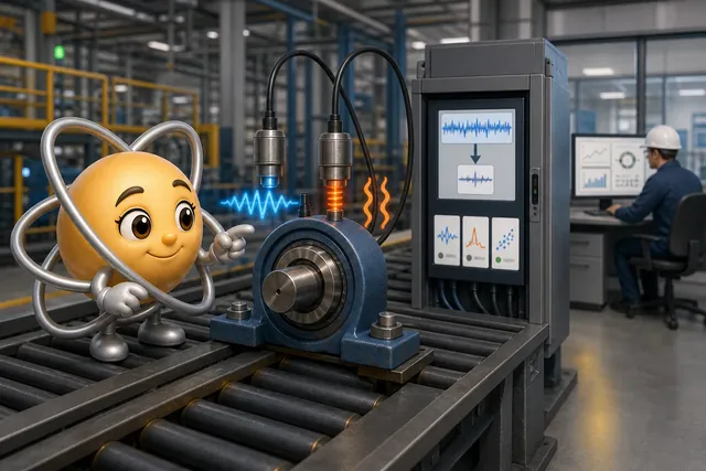
Ada gathers condition evidence from the bearing.
-
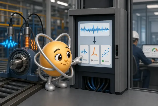
The edge device turns the signal into useful features.
-
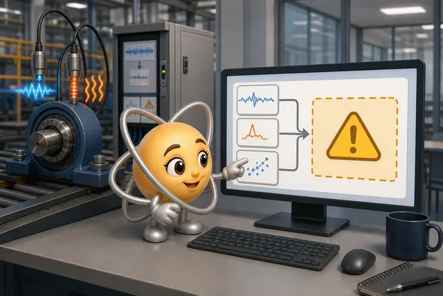
Analytics estimate fault type and severity.
-
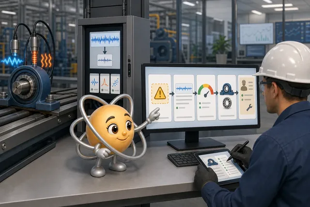
The warning becomes a reviewable work order.
-
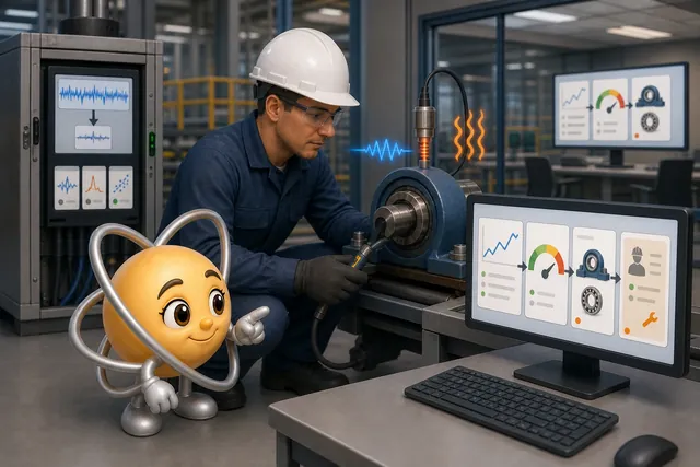
The technician result returns to the evidence loop.
Each hand-off must preserve enough context for the next person to review the result. A feature window without its source conditions breaks that chain, even if the dashboard continues to show a score.
This diagram uses concrete example values to show where data volume changes. Treat the numbers as a design scenario that must be replaced by measured asset data in a real deployment.
The path to watch in Figure 5 is the red one along the bottom, which shows what is lost when a stage is skipped.

Start at sensing in Figure 5. The waveform is captured fast enough to hold bearing detail, and the operating context travels with it. The edge stage turns that raw window into a few named features and records how they were produced, so a later reviewer can tell a real change from a settings change. Analytics compare those features with a baseline and attach the evidence to an alert, but the figure is blunt about the limit: a pattern shows that something changed, not why. The workflow stage closes the loop by returning the technician’s finding. Now follow the red bypass. Sampling straight at one reading per second removes the frequencies the diagnosis depends on, and no later stage can bring them back.
31.9 Read Vibration as Fault Evidence
Rotating machinery (motors, pumps, fans) reveals health through vibration signatures:
Inspect Figure 6 to see how one vibration sample supports different time- and frequency-domain fault tests.

Read Figure 6 from three-axis sampling into the parallel analysis paths. RMS and peak describe overall and maximum motion; crest factor divides peak by RMS to expose impulsive events. The FFT and order analysis locate components tied to shaft speed, while envelope analysis demodulates high frequencies that reveal bearing faults. The final signatures give the physical interpretation: imbalance near 1× shaft speed, misalignment near 2×, and bearing peaks at BPFO, BPFI, BSF, or FTF harmonics. Compare each peak with a baseline before calling it a defect.
The illustrated three-axis sensing range is 100–1000 Hz. That example is not sufficient for every bearing diagnosis: choose sampling bandwidth for the required fault evidence, rather than copying a dashboard rate.
The fault signatures below guide the next inspection; they do not establish a diagnosis alone.
| Defect | Frequency Signature | Detection Lead Time |
|---|---|---|
| Imbalance | 1x shaft speed | Estimate lead time from this asset’s vibration trend and operating load |
| Misalignment | 2x shaft speed (axial and radial) | Assess urgency from severity, trend and load |
| Bearing defects | BPFO, BPFI, BSF, FTF harmonics | Estimate from trend, severity and operating load |
| Gear mesh | Teeth count x shaft speed | Estimate from trend, severity and operating load |
| Looseness | Multiple harmonics, random spikes | Estimate from trend, severity and operating load |
Choose the analysis for the evidence needed.
In time-domain analysis, RMS describes overall vibration, peak records the maximum amplitude, and crest factor divides peak by RMS to expose impulsive events. These features describe the waveform without locating a particular frequency component.
Frequency-domain analysis separates components. The fast Fourier transform identifies frequencies to compare with defect signatures. Order analysis tracks components relative to shaft speed, while spectral trending monitors changes in selected frequency bands over time. Compare those changes with a baseline taken under known operating conditions.
For more complex evidence, envelope analysis demodulates high-frequency motion to reveal bearing faults. Wavelet analysis keeps time and frequency information together for transient events. Cepstrum analysis looks for periodic patterns in the spectrum, including gear families. Choose among these methods according to the failure mechanism and the evidence preserved by sampling.
Set the response timeline from the asset, rather than from a generic number of days.
| Defect Type | Early Detection | Actionable Alert | Critical |
|---|---|---|---|
| Bearing wear | Establish from asset trend | Set from severity and criticality | Use site alarm limits |
| Imbalance | Establish from asset trend | Set from severity and criticality | Use site alarm limits |
| Misalignment | Assess from severity, trend and load | Set from asset evidence | Use site alarm limits |
| Lubrication | Establish from asset trend | Set from severity and criticality | Use site alarm limits |
For a pump motor, a stable dominant 2× shaft-frequency component in both axial and radial directions points the next inspection toward shaft misalignment when bearing-defect frequencies and multiple looseness harmonics are absent and mounting bolts are tight. Confirm alignment mechanically. In the changed case, a dominant 1× radial component with the same absent signatures instead points toward uneven rotor mass and imbalance. Neither spectrum removes the need for inspection.
BPFO is ball-pass frequency at the outer race; BPFI is ball-pass frequency at the inner race. BSF denotes ball-spin frequency, and FTF denotes fundamental train frequency. Geometry and speed place these bearing components at different frequencies, while trend, harmonics, severity, and load determine their significance.
At 1,780 rpm, a nine-ball bearing with a 0.30 ball-to-pitch diameter ratio places its outer-race fault near 93.5 Hz and inner-race fault near 173.6 Hz. A 10 kHz waveform preserves both below its 5 kHz Nyquist limit. A 1 Hz dashboard trend can fold these components into slow aliases near 0.45 Hz and cannot preserve the original diagnostic evidence. Sampling choices must therefore precede a claim about what a model can detect.
The separate vibration simulation uses a different bearing: eight balls, 0.5-inch ball diameter, 3.0-inch pitch diameter, and zero-degree contact angle. Its shaft-speed control spans 10–100 Hz in 5 Hz steps, starting at 30 Hz. Keep those example geometries separate when interpreting BPFO and BPFI.

The Simulations Hub offers further vibration and FFT visualization tools. Use the Videos Hub for predictive-maintenance and smart-factory implementation examples after identifying which physical evidence each example actually shows.
31.10 Check the Installation and Close the Loop
Vibration is one condition signal; thermal imaging adds a physical inspection perspective. Compare the infrared cameras below by package, exposed interfaces, mounting, scale, and service access before treating their forms as interchangeable.


Read across the forms as engineering evidence. They share a capability name, but packaging and installation change the electrical, mechanical, environmental, and maintenance constraints.
Start with a small group of machines and count useful warnings, false alarms, missed faults, saved stops, and needless work. Scale only when the evidence and workflow earn technician trust. Add one machine type at a time, train the warning recipients, and keep a return path. Check every shift, quiet and busy work, heat and cold, and recovery after power loss. Keep the old method until the new path has proved dependable.
For remaining-useful-life training and evaluation, link time-stamped asset feature windows to confirmed fault dates and observed outcomes. A dashboard score alone has no observed lifetime; an anomaly is not a confirmed failure date. Dropping asset identity or operating context prevents a reliable match between windows and life history. This closes the evidence chain needed by the next chapter’s models.
Summary
Predictive maintenance connects a named failure mode to a measurable signal and an owned response. Criticality determines where monitoring is worth its cost; operating context and feature lineage make the evidence reviewable. Raw windows, derived features, alerts, and technician findings must remain linked so confirmed faults and false alarms can improve the system.
Vibration features help direct an inspection. RMS, peak, and crest factor describe motion; frequency and envelope methods expose patterns tied to shaft speed or bearing geometry. Detection and response windows depend on the asset’s trend, severity, load, and site limits. The business case must include inspection costs and ongoing operation as well as any avoided downtime.
Choose the fault and maintenance action first, then preserve the signal and context needed to justify that action. A warning creates value when a technician can review it and complete planned work.