3 Manufacturing IoT: OT Integration Boundaries

3.1 Start With the Decision

Test evidence should follow the complete loop, not just the device.

3.2 Route Overview

This is part 2 of 2. Review Manufacturing IoT: Connected Factory Systems for the preceding evidence.

3.3 Learning Objectives

• Test ot integration boundaries with a concrete scenario and pass criteria.
• Validate putting numbers to it with a concrete scenario and pass criteria.

3.4 Chapter Roadmap

• OT Integration Boundaries
• Motion Marley’s Math Bridge: Sample Rate to FFT Evidence
• Checkpoint: Plant Decision Loop
• The Four Pillars of Smart Manufacturing
• Quick Check: Closing the Factory Loop
• CNC Predictive Maintenance
• Remote Food Safety Recalls
• Smart Packaging Active Sensing
• Putting Numbers to It
• Checkpoint: Packaging Evidence
• Continue to Part 2

3.5 OT Integration Boundaries

A plant prototype must respect that production systems run under availability, safety, quality, cybersecurity, and change-control constraints. The safest prototype often reads first, writes later, and proves how data will be governed before it is allowed to affect control.

Under the hood, the hard problem is usually not the sensor driver; it is preserving meaning across layers. A PLC tag such as MTR_07_VIB_RMS may be sampled every second at the edge, compressed by a historian, joined to a motor asset in a CMMS, associated with a batch in MES, summarized into an OEE dashboard, and used by finance to justify a spare-parts policy. If any layer changes the unit, timestamp, asset id, threshold, or missing-data rule without control, the final decision can be wrong even though every individual system appears healthy.

Safety and cybersecurity boundaries must be explicit. Telemetry that only informs maintenance can often be read through OPC UA, MQTT, or a historian interface with limited risk. Control writebacks, recipe changes, and interlocks require stronger review because they can affect equipment, operators, product quality, and regulatory records. In IEC 62443 terms, the design should define zones, conduits, trust relationships, remote-access controls, certificate rotation, account ownership, patch windows, logging, and rollback. In production terms, the design should define who is allowed to acknowledge an alarm, override a recommendation, release a held batch, or defer a work order.

Test evidence should follow the complete loop, not just the device. A useful acceptance test injects a known bearing-fault pattern, verifies edge feature extraction, checks the timestamp in the broker and historian, confirms the MES or CMMS action, observes the operator response, and records whether downtime, scrap, energy, or quality actually improved. That loop-level evidence is what separates a factory demo from a deployable manufacturing system.

• Control boundary: separate read-only telemetry, advisory alerts, operator-approved actions, PLC writebacks, interlocks, and safety-instrumented functions.
• Data boundary: version tag names, units, sampling intervals, deadbands, timestamp source, historian compression, batch context, and missing-data behavior.
• Cyber boundary: define IEC 62443 zones and conduits, OT DMZ, firewall rule, broker certificate, user role, remote-access policy, and patch window.
• Change boundary: define who approves tag additions, recipe changes, dashboard thresholds, MES mappings, CMMS workflow changes, and rollback after a bad deployment.

The prototype is stronger when one event can be traced from sensor or PLC tag through edge gateway, broker, historian, MES/ERP/CMMS action, operator response, and measured production outcome.

3.6 Motion Marley’s Math Bridge: Sample Rate to FFT Evidence

The mathematical gist. A 10.0 kHz sample rate has a 5.00 kHz Nyquist limit. A 1,024-sample FFT spans 102.4 ms with 9.77 Hz bins, placing the chapter’s 1,800 Hz tone near bin 184. A hypothetical 6.20 kHz component folds to 3.80 kHz, while a 16-bit ±5g input has a 0.000153g step—so sample timing, not amplitude resolution, sets this example’s main evidence risk.

Math Bridge · guided foundationsWhy does a 10 kHz sample clock stop the FFT at 5 kHz?Let Motion Marley connect sample rate, window length, bin width, aliasing, and quantisation. Learn the maths

3.7 The Four Pillars of Smart Manufacturing

• Manufacturing Plant: Capabilities: Real-time production monitoring, waste elimination, condition-based maintenance alerts; Business Value: Increase throughput, reduce unplanned downtime
• Global Facility Insight: Capabilities: Remote equipment management, temperature/energy optimization; Business Value: Cut energy costs 15-25%, manage multiple facilities centrally
• Customer Site: Capabilities: Transmit operational data to OEM, enable remote service; Business Value: Faster repairs, proactive parts replacement
• Global Operations: Capabilities: Cross-site visibility, usage analytics, depreciation tracking; Business Value: Optimize capital allocation, predict maintenance needs

Figure 3.1 shows what changes as the same plant data travels further from the machine that produced it.

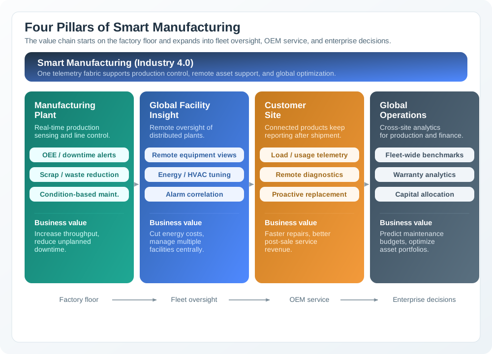
Read the four columns left to right and watch the distance grow. The first stays inside one plant, where data controls a line in real time. The second steps back to several sites, where the same feeds become energy and alarm comparisons. The third leaves the company: the product now sits at a customer site, and telemetry supports service rather than production. The fourth sits with finance, where fleet-wide patterns shape warranty and capital decisions. Notice that every column pairs a capability with a business value, and that the band across the top names a single telemetry fabric. Figure 3.1 argues that these are one investment read at four ranges, not four separate projects.

3.8 Quick Check: Closing the Factory Loop

3.9 CNC Predictive Maintenance

Let’s trace how a smart factory detects an impending bearing failure 10 days before catastrophic breakdown:

Before trusting a vibration spectrum, look at what produced it: Figure 3.2 cuts one sensor open.

Start at the top of the housing. The coarse screw thread is not a convenience, it is the signal path, because a stud joint is stiff enough to pass fast machine motion into the sensor without smearing it. Below it, the hex flats show that the part is meant to be tightened to a set value, so fitting is a specified step rather than a habit. The cut-away window in the middle reveals the short stack of discs clamped inside the solid metal body, which is the sensing element and its mass. Figure 3.2 explains why the maintenance record must state where and how the sensor was mounted, not just what the spectrum showed.

Step 1: Sensing (Machine Layer)

• Triaxial vibration sensor mounted on CNC milling machine spindle housing
• Accelerometer samples at 10 kHz (10,000 readings/second) in X, Y, Z axes
• Industrial temperature sensor monitors bearing housing (every 1 second)
• Current sensor on motor power line detects electrical anomalies (every 100 ms)

Step 2: Edge Processing (PLC/Edge Gateway Layer)

• Edge computer attached to machine performs Fast Fourier Transform (FFT) on vibration data
• Converts time-domain acceleration signal to frequency spectrum (0-5000 Hz)
• Identifies dominant frequency peaks: 60 Hz, 120 Hz, 1800 Hz, 3600 Hz
• Normal bearing: Vibration energy concentrated at 1800 Hz (spindle rotation frequency)
• Degraded bearing: New peaks appear at bearing fault frequencies
  • Inner race fault: appears at 1800 + (1800 x 0.042) = 1875.6 Hz
  • Outer race fault: appears at 1800 - (1800 x 0.035) = 1737.0 Hz
  • Ball defect: appears at 1800 x 0.021 = 37.8 Hz sidebands

Step 3: Anomaly Detection (Edge ML)

• Edge ML model (trained on 2 years of historical data from 50 identical machines) compares current spectrum to baseline
• Fault severity score: 0-100 (0 = healthy, 100 = imminent failure)
• Current reading: Severity = 35 (yellow zone, schedule maintenance)
• Trend analysis: Severity increased from 10 to 35 over past 7 days (linear progression predicts severity 70 in 10 days)

Step 4: ERP Integration (Enterprise Layer)

• Edge gateway sends alert to Manufacturing Execution System (MES): “Machine CNC-07 bearing fault detected, predicted failure in 10 days”
• MES checks production schedule: CNC-07 has planned downtime in 8 days for tool change
• MES automatically orders replacement bearing from supplier (SKU: FAG-6205-2RSR, $45, 3-day delivery)
• Work order generated for maintenance team: “Replace spindle bearing during scheduled downtime on Day 8”

Step 5: Outcome

• Bearing replaced during 4-hour planned maintenance window
• Avoided cost: Unplanned breakdown would have caused 48-hour production halt ($120K revenue loss) + emergency bearing ($200, expedited) + overtime labor ($500) + damaged spindle ($8K)
• Actual cost: Planned bearing replacement ($45 part + $200 labor during normal downtime) = $245
• ROI: $128K avoided cost / $245 actual cost = 523× return on predictive maintenance intervention

Key Insight: The vibration sensor didn’t prevent the failure — the integration with MES did. Without MES integration, the maintenance team would have logged the alert but taken no action because they didn’t know the production schedule allowed early intervention.

Common Failure Point: Many factories install vibration sensors but send alerts only to a separate “condition monitoring dashboard.” Maintenance teams check it weekly, by which time the bearing has already failed. The sensor data is correct, but the workflow integration is wrong.

3.10 Remote Food Safety Recalls

A powerful but underappreciated IoT capability: connected products that can refuse to work when safety issues arise.

The same pattern can begin on the production line. A machine-vision check can detect a faulty food packet and stop the machine from pressing or sealing that packet. Detection alone is not the control outcome: the design must connect the inspection result to the interlock that prevents the next unsafe process step.

Example: When a produce recall is issued, a connected juicer can:

1. Check QR codes on ingredient packs against recall database
2. Prevent pressing of affected batches
3. Alert user to return affected products
4. Provide manufacturer with real-time recall compliance data

Why This Matters:

• Traditional recalls rely on customers hearing news and checking pantries
• IoT-connected products can actively prevent consumption of recalled items
• Manufacturer gets instant visibility into recall effectiveness
• Particularly critical for infant formula, medications, allergens

3.11 Smart Packaging Active Sensing

Figure 3.3 answers the cost question behind smart packaging: how much hardware does a package actually have to carry?

Look first at the ruler along the bottom. The whole tag is about three centimetres across and flat enough to sit under a printed label, which is what makes one per package affordable. Now follow the spiral of printed tracks inward. Those loops are the antenna, and they are also the power supply, because the reader’s field is what wakes the tag. There is no battery to fit or replace. At the centre sits the only silicon in the device, a chip far smaller than the coil that feeds it. Figure 3.3 sets the honest baseline here. Identity travels cheaply, while active sensing has to earn its extra cost.

Smart packaging systems for food and pharmaceuticals go beyond passive containment to actively sense, measure, communicate, and respond to product conditions.

The Shift from Passive to Active Packaging:

• Function: Traditional Packaging: Contain and protect; Smart/Active Packaging: Sense, communicate, respond

• Information: Traditional Packaging: Static label (printed date); Smart/Active Packaging: Dynamic data (actual freshness)

• Shelf life: Traditional Packaging: Conservative estimates; Smart/Active Packaging: Real-time remaining quality

• Temperature abuse: Traditional Packaging: Unknown until spoilage; Smart/Active Packaging: Logged and visible

• Consumer trust: Traditional Packaging: “Best by” guess; Smart/Active Packaging: Verified quality chain Smart Packaging Technologies:

• Time-Temperature Indicators (TTI): What It Monitors: Cumulative heat exposure; Use Cases: Cold chain integrity for vaccines, seafood

• Freshness Indicators: What It Monitors: CO2, ammonia, volatile amines; Use Cases: Meat, fish spoilage detection

• Oxygen Indicators: What It Monitors: O2 levels in modified atmosphere; Use Cases: MAP (Modified Atmosphere Packaging) integrity

• RFID/NFC Tags: What It Monitors: Product identity, temperature log; Use Cases: Supply chain tracking, authentication

• Printed Electronics: What It Monitors: Moisture, pH, bacterial contamination; Use Cases: Pharmaceutical blister packs Economic Opportunity:

• 30% of food wasted globally due to conservative “best by” dates

• $35 billion in US pharmaceutical waste annually from discarded “expired” medicines

• Vaccine cold chain failures cause 25% of vaccines to arrive degraded

• Counterfeit drugs worth $200 billion/year could be detected with authentication packaging

• Smart packaging market projected to reach $46 billion by 2030

3.12 Putting Numbers to It

A pharmaceutical distributor ships 500,000 vaccine doses per year at $45 per dose. If 25% arrive degraded because of cold-chain failures, annual waste is 500,000 x 0.25 x $45 = $5,625,000.

Time-Temperature Indicator (TTI) smart packaging costs $0.85 per dose, including the tag and cloud logging. If that monitoring reduces degradation to 3%, the new waste is 500,000 x 0.03 x $45 = $675,000, and the packaging program costs 500,000 x $0.85 = $425,000.

Net annual savings are $5,625,000 - $675,000 - $425,000 = $4,525,000. The payback period is $425,000 divided by $4,525,000 / 12, or about 1.1 months. After payback, the monthly benefit is approximately $377,000.

3.13 Continue to Part 2

Continue with Manufacturing IoT: Maintenance and Supply Chains.

3.14 Continue Your Route

This final part closes the route from OT Integration Boundaries through Continue to Part 2. Return to Manufacturing IoT: Connected Factory Systems or continue from the applications module index.